Structural Priors Learning
Context
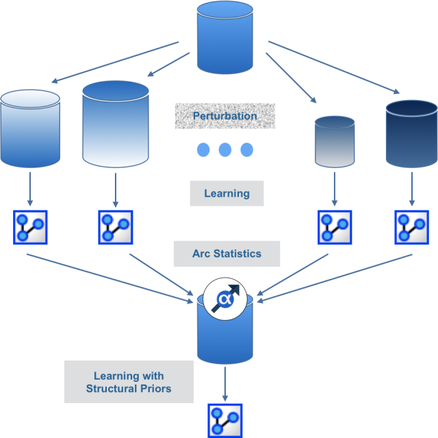
Structural Priors Learning is a Meta-Learning algorithm that can be compared to Bagging. It is based on Data Perturbation (Smoothed Bootstrapping) for learning a bag of networks and gathering statistics about the relationships that have been found. These statistics are then used for automatically defining Structural Priors.
Once defined, the Structural Priors are used for learning a network on the original unperturbed data set.
Example
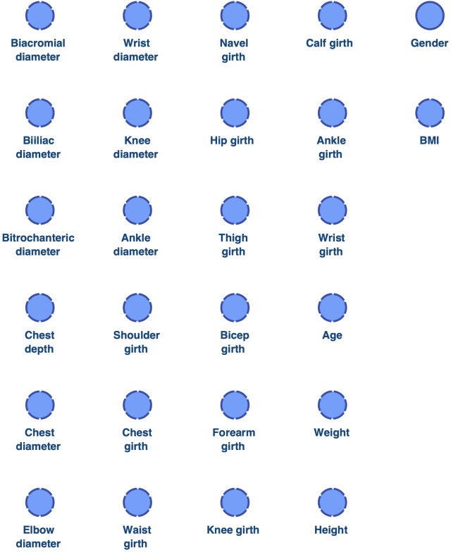
Let’s use a small data set that contains only 91 particles. Each particle is a physically active individual (several hours of exercise a week), described with body girth measurements and skeletal diameter measurements, as well as age, weight, height, and gender.
All the variables are continuous, except . We discretized all continuous variables with R2GenOpt* 3.
We define Temporal Indices to specify that Age and have to be root nodes.
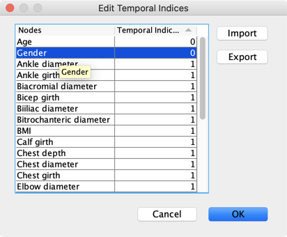
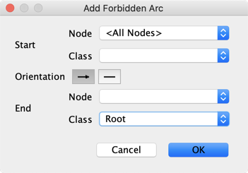
The same result can be obtained by associating these two nodes in a class and then forbidding incoming arcs to this class.
Below is the network learned with EQ.
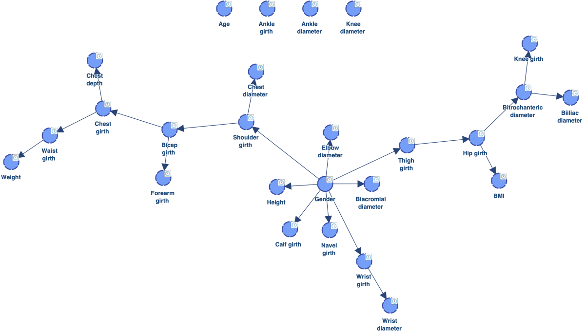
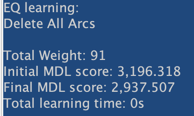
Let’s use Data Perturbation in order to try to escape from the local optima found with EQ.
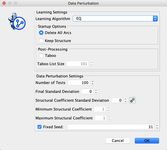

The obtained network has a better score than the one obtained with EQ. It also makes more sense, as we can see that it captures the relationship between Weight, Height and BMI.
However, we still have four “orphan” nodes: Ankle diameter, Ankle girth, Age and Knee diameter. There are two scenarios: either these nodes are really marginally independent of all the other nodes, or their relationships with the other nodes are above the “significance threshold” implicitly defined by the MDL score.
Keeping in mind that we just have 91 particles, and given that the MDL score is conservative, we can try decreasing the Structural Coefficient.
Instead of manually testing the structural coefficient, we use the Structural Coefficient Analysis tool.

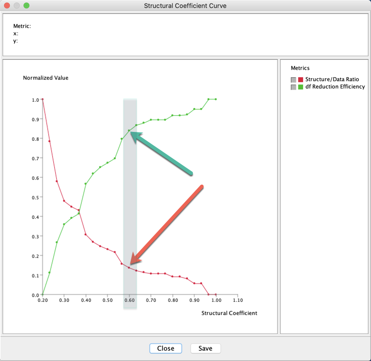
The analysis of these curves suggests the utilization of a Structural Coefficient = 0.6.
The network below has been learned with Data Perturbation - EQ.
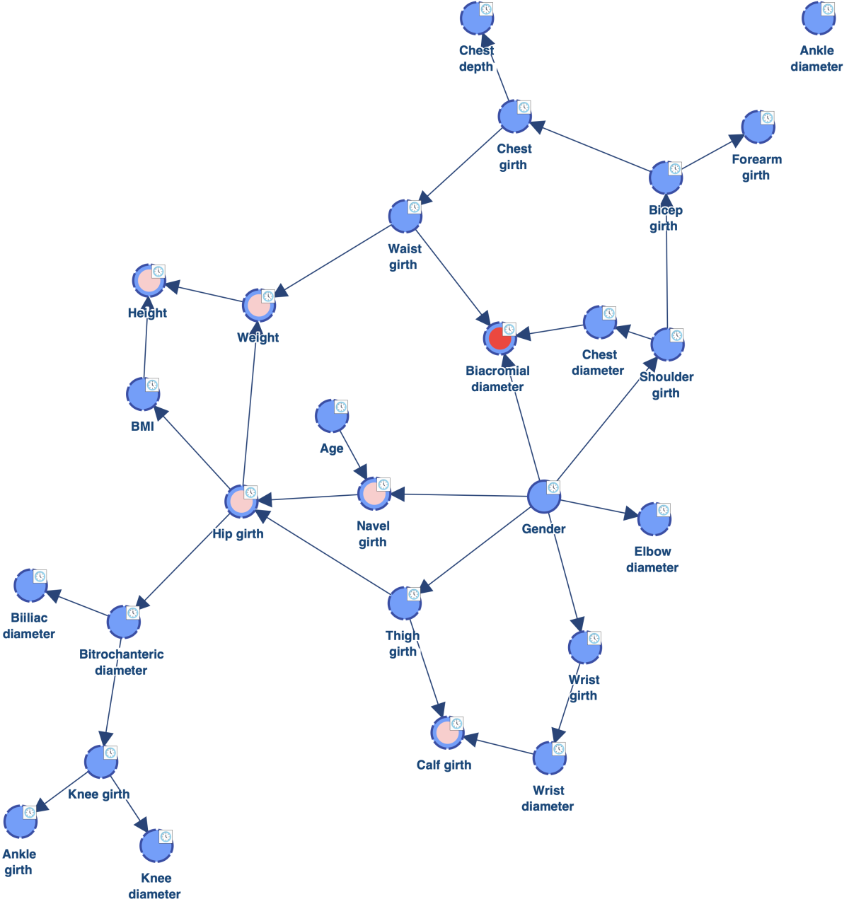
As we can see, there is now only one orphan: Ankle diameter. Reducing the value of the Structural Coefficient was indeed efficient for connecting the orphans. However, this coefficient has a global impact on the MDL score. It reduces the cost of adding arcs for all the nodes. We can see for example that Biacromial diameter (highlighted in red) has now three parents, which is probably too much given the amount of data available. There are also now five nodes with two parents (highlighted in pink), instead of one with the Structural Coefficient = 1.0.
Instead of reducing the Structural Coefficient globally, we now use Structural Priors Learning for exploring a range of coefficients [0.2 ; 1.0] and automatically get Structural Priors.

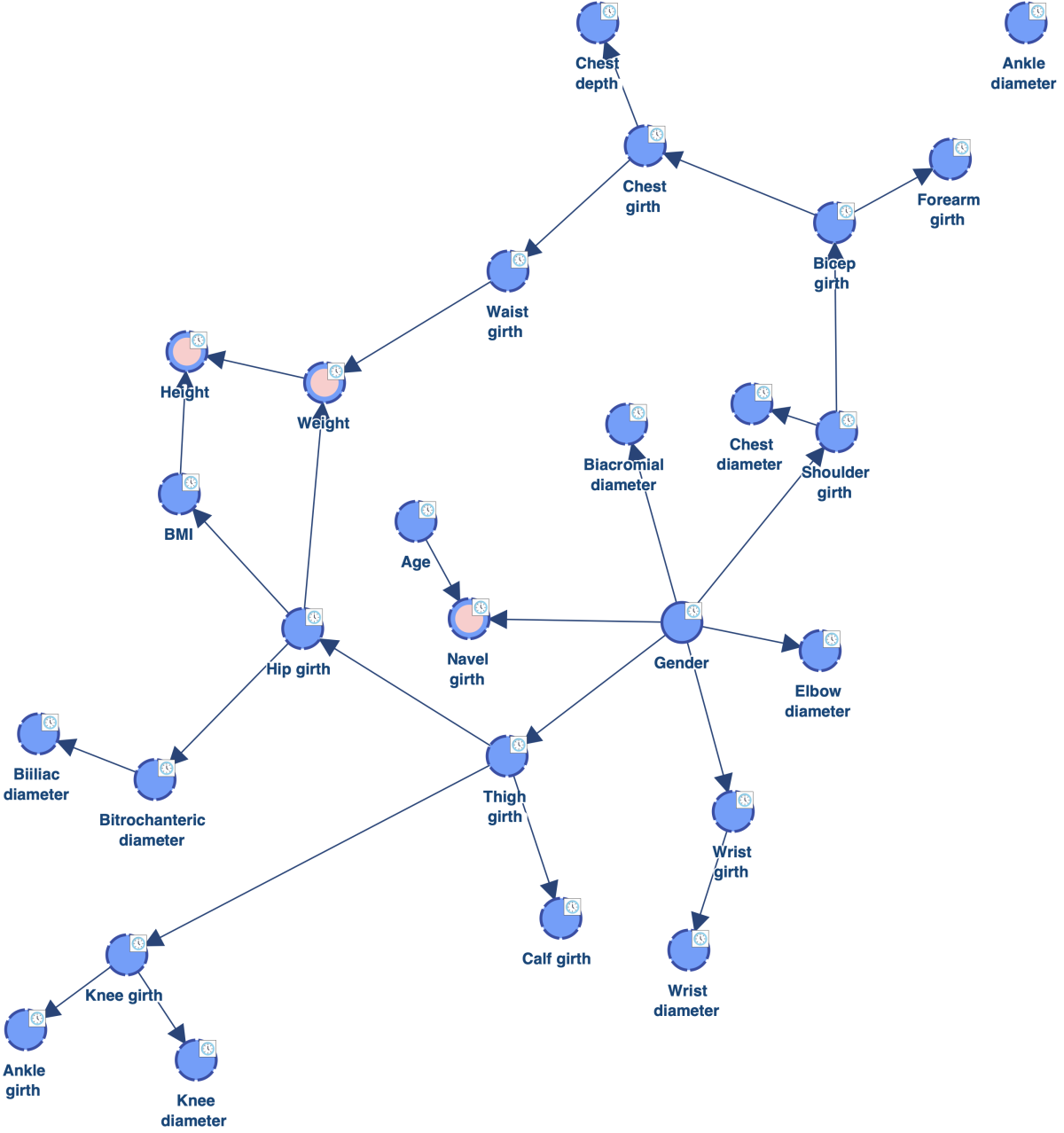

In addition to the MDL score, the Console  returns the
 Min, Max, and Mean of the arcs’ Priors that are represented in the learned network.
As we can see, there is also only one orphan. However, the complexity of the obtained network is lower than the one learned with a Structural Coefficient = 0.6. The Biacromial diameter has only one parent, which makes much more sense given the amount of data available, and there are only three nodes with two parents (highlighted in pink).
Clicking  in the lower right corner of the graph window opens the editor of the Structural Priors.
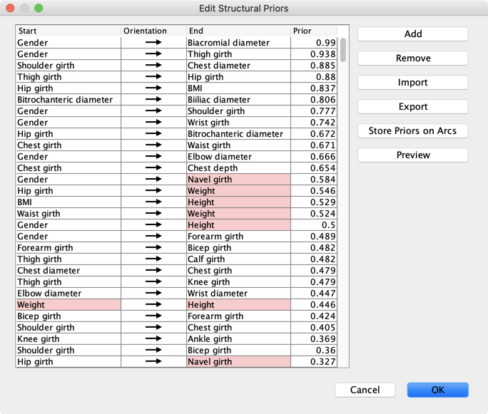
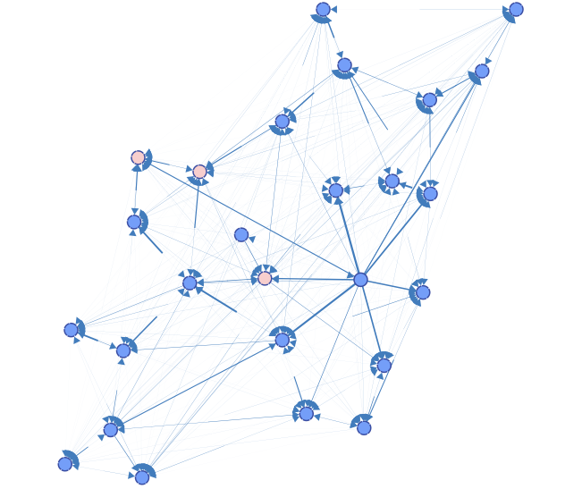
The Preview returns a graph with all the connections that have been learned on the perturbed data sets.
Store Priors on Arcs associates the priors with the arcs of the network. It is also a way to get in the Console the Min, Max, and Mean of the arcs’ Priors that are represented in the current network.