
Curve
Context
The Curve window is a key element of the Structural Coefficient Analysis, from where it can be launched.
Usage
You can open the Curve window by clicking the Curve button at the bottom of the Structural Coefficient Analysis Report.
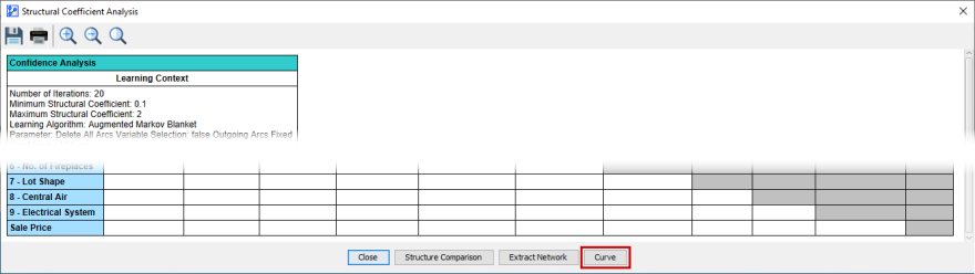
Curve Window
-
Depending on what you selected in Analysis Settings at the beginning of the Structural Coefficient Analysis and what type of network you have, a range of metrics is available to plot.
-
All of them are shown simultaneously in the following screenshot. In practice, you would view them individually, and only some might apply to your analysis context.
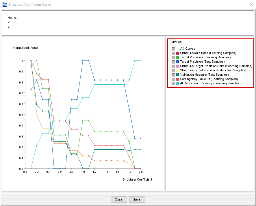
Metrics Interpretation
We explain each metric in a dedicated section with an example:
- Contingency Table Fit
- Structure/Data Ratio
- Degree of Freedom Reduction Efficiency
- Structure/Target Precision Ratio
- Target Precision
- Validation Measure
- The Target Precision measure is exclusively available with networks that feature a Target Node.
- If the dataset is split into a Learning Set and a Test Set, Target Precision is computed separately for each set for each value of the Structural Coefficient.
- The measures are plotted on a normalized basis, like the Structure/Data Ratio.
Structural Coefficient Analysis (7.0)
Context
Tools | Multi-Run | Structural Coefficient Analysis
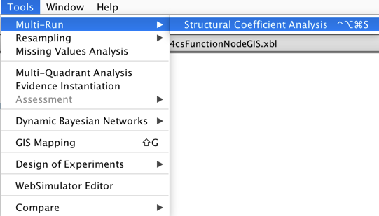
This tool helps choose the best Structural Coefficient by testing structural learning algorithms with a range of coefficients, which impacts the structural complexity of the machine-learned networks.
Renamed Menu Item
This feature was previously under Tools | Cross-Validation.
New Feature: Rediscretize Continuous Nodes
This option allows running automatic discretization before executing the selected structural learning algorithm with the current Structural Coefficient.
The discretization runs only for continuous variables that have an associated automatic discretization algorithm, i.e., for which the discretization thresholds have not been manually defined (or modified). Note that the Target Node is never rediscretized in this context.
The main purpose of this option is to allow testing the impact of the Structural Coefficient on the discretization algorithms. It is thus geared toward supervised learning problems, where the variables are discretized with Tree-based approaches. The Structural Coefficient is also used in the MDL score that is utilized for the induction of the trees.
However, if the Seed is not fixed, this can also affect the following discretization algorithms that are stochastic by nature:
Example
Let’s use a dataset that contains house sale prices for King County , which includes Seattle. It describes homes sold between May 2014 and May 2015. More precisely, we have extracted the 94 houses that are more than 100 years old, that have been renovated, and come with a basement.
All the continuous variables have been discretized into three bins, with R2-GenOpt.
Given the small number of observations in this dataset, we set five prior samples for the Smoothed Probability Estimation (5.0.4) in order to use a non-informative prior in the estimation of the parameters.
Below is the network learned with EQ and the default Structural Coefficient:
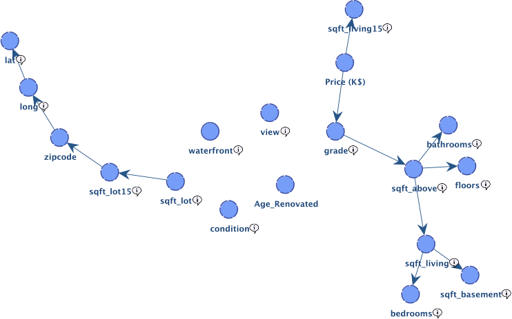
Four nodes remain unconnected.
This means that, from the MDL score perspective, with the default Structural Coefficient, relationships with the other nodes are too weak, and therefore it is “too expensive” to represent these relationships. In other words, the additional bits required to represent the structure, if we were to add a link with one of these nodes, will not be compensated by the reduction in the number of bits needed to represent the data.
One way to try getting these nodes connected would be to decrease the number of bins used for discretization. This would automatically reduce the “price” for adding links with these nodes.
However, if we want to keep the same discretization, we can try to reduce the Structural Coefficient. Instead of manually selecting a value by trial and error, the Structural Coefficient Analysis tool can be used for automatically testing different coefficients.
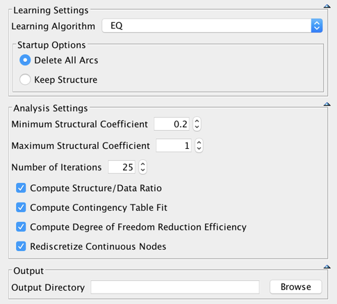
With this setting, 25 networks are learned with EQ, starting with a Structural Coefficient = 1, then to 0.968, then 0.936 …, the last network being learned with a Structural Coefficient = 0.2.
Prior to each trial, the nodes are discretized into three bins with R2-GenOpt. As the seed of our random number generator is fixed, unchecking Rediscretize Continuous Nodes would return the exact same results.
The three selected metrics are computed for each of these 25 networks.
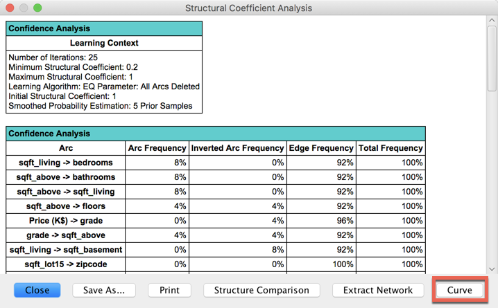
The normalized values of these metrics are available by clicking the Curve button:
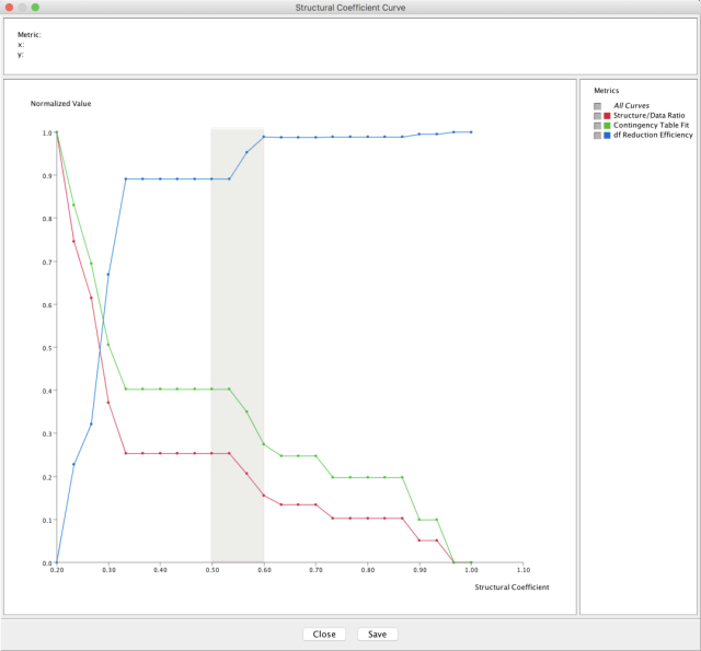
All these curves suggest a coefficient between 0.5 and 0.6.
Updated Feature: Structure Comparison
Comparing the structure of the learned networks usually helps to decide which coefficient to finally use. The networks are now stored from the largest Structural Coefficient to the smallest.
Example
Let’s continue with our house example. The structures of the networks can be compared by clicking Structure Comparison.
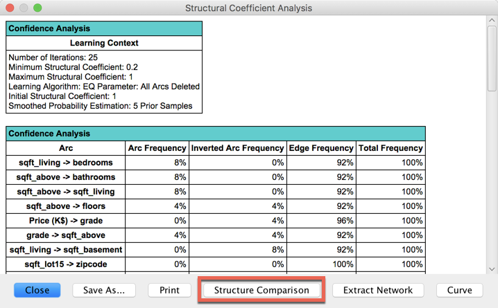
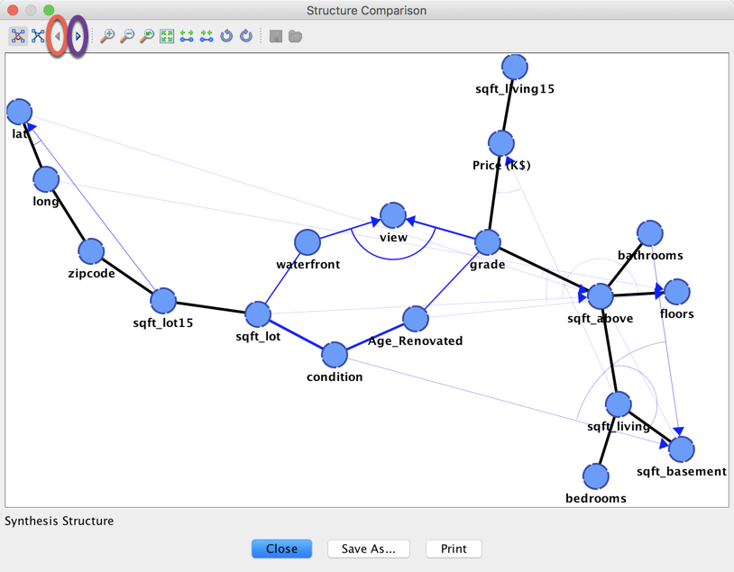
The two highlighted arrows are used to go through the different structures.
- Synthesis Structure
- Reference Structure
- Max SC = 1
- Max SC = 0.933
- Max SC = 0.6
- Max SC = 0.567
- Max SC = 0.533
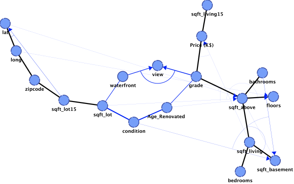
The Synthesis Structure is not a Bayesian network. It is a graph that contains all the links that have been generated during the different trials.
A link can have three different colors:
- Black: the link belongs to the initial structure and has been found in at least one generated solution.
- Red: the link belongs to the initial structure but has never been found in the generated solutions.
- Blue: the link does not belong to the initial structure but has been found in at least one generated solution.
Furthermore, the thickness of the link is proportional to its frequency in the generated structures.
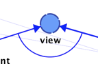
When an arc is added between two nodes, this indicates a V-Structure. Without an arc, the link can have both orientations in its Equivalence Class.
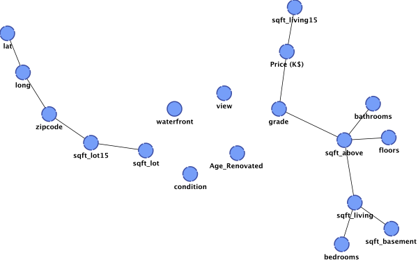
This is the network shown in the Graph Panel when the analysis is run.
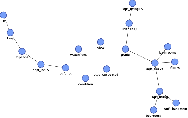

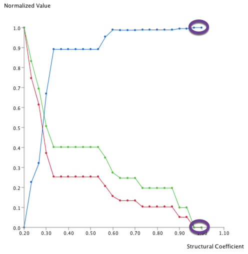
This structure has been found twice, and the maximum Structural Coefficient was 1. They correspond to the two highlighted points in the graph below:
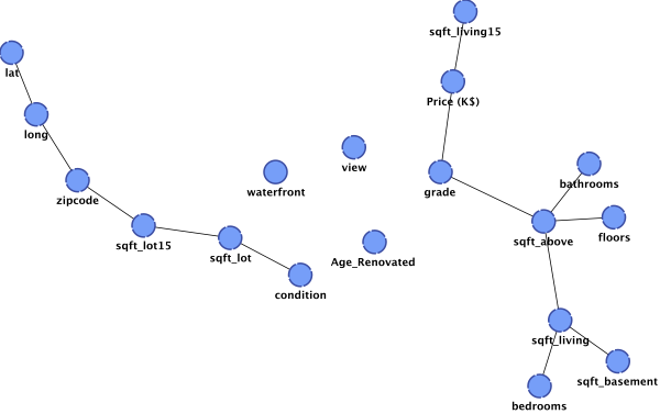

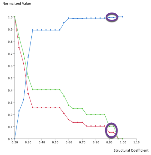
This structure has been found twice, and the maximum Structural Coefficient was 0.933. They correspond to the two highlighted points in the graph below:
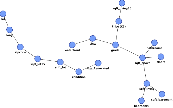

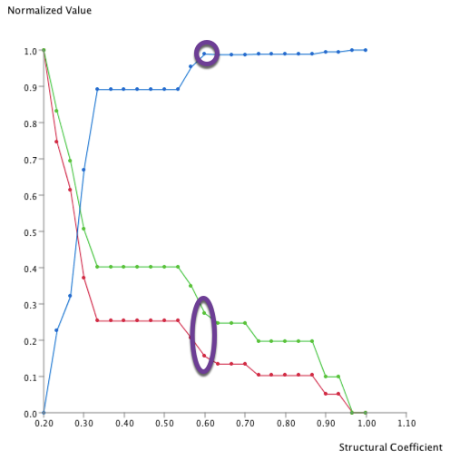
This structure has been found once with a Structural Coefficient = 0.6. It corresponds to the highlighted point in the graph below:
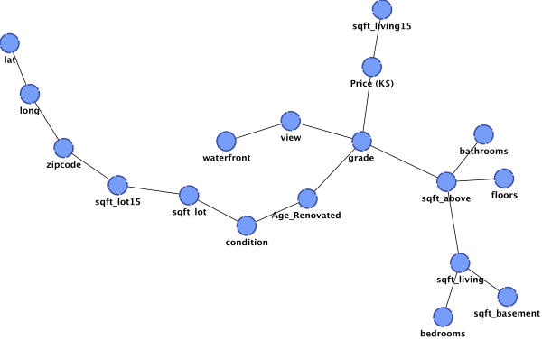

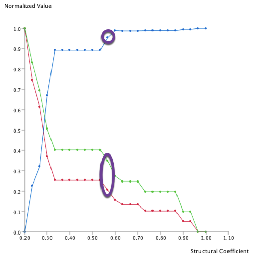
This structure has been found once with a Structural Coefficient = 0.567. It corresponds to the highlighted point in the graph below:
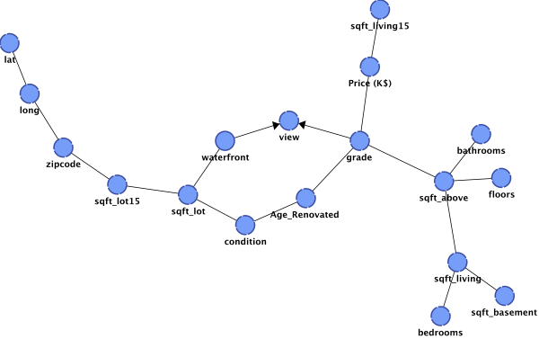

This structure has been found seven times, and the maximum Structural Coefficient was 0.533. They correspond to the highlighted points in the graph below:
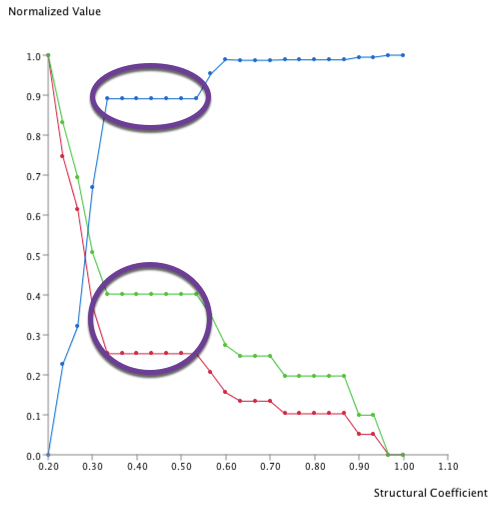
Given these structures, a conservative choice would be to select the solution with a path between every node and the largest coefficient, i.e., the solution with a Structural Coefficient set to 0.567.
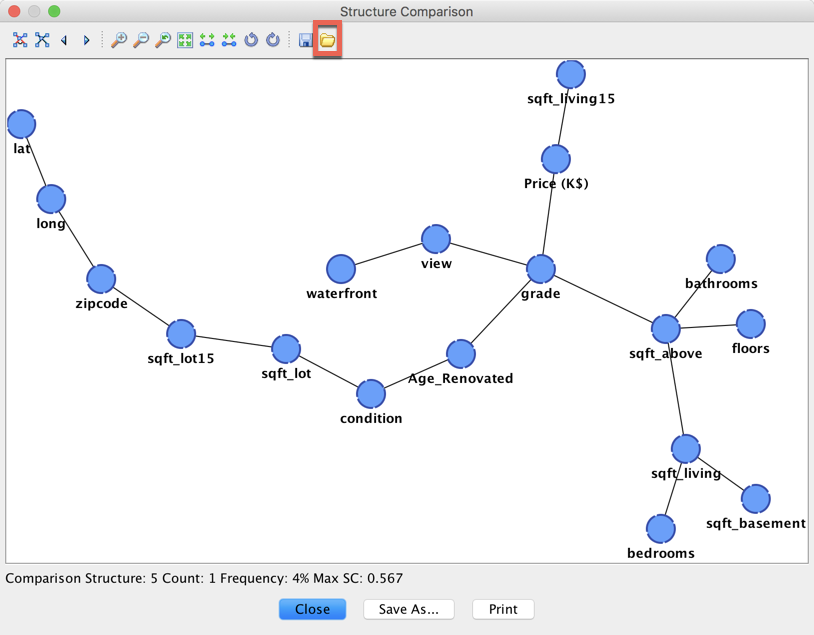
Clicking the highlighted icon  allows you to directly open a new graph with the visualized structure.
When choosing a Structural Coefficient lower than 1, it is highly recommended to double-check that the relationships represented by decreasing the Structural Coefficient are significant. This can be done by running Analysis | Report | Relationship.
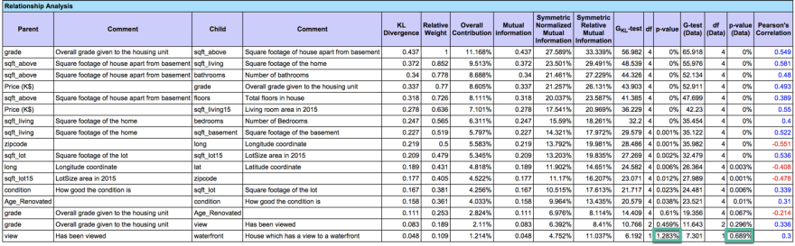
The p-value highlighted in green confirms that the relationships are significant with a threshold set to 1%. Note that, even though there is a link between view and waterfront, the p-value computed with the model and the one computed directly on the data (assuming a direct link between the two variables) are not exactly the same. This is because the model has been learned with five prior samples for the Smoothed Probability Estimation, thus slightly smoothing the relationship.
Doing the same analysis on the network learned with a Structural Coefficient set to 0.533 returns a p-value of 2% for the weakest relationship estimated on the data.