Prediction Analysis

Context

The Prediction Analysis tool allows you to examine the predictive performance of a network model interactively. It generates a new causal network to represent the performance dynamics of the original model. This approach can help you interpret concepts such as precision, reliability, true/false positives, true/false negatives, etc. As a result, the usefulness of the model can be assessed and explained in detail.

Usage & Example

Before you can initiate a Prediction Analysis, you need to have a network that was learned using Supervised Learning. Ideally, you would perform all other validation and performance testing steps, e.g., Structural Coefficient Analysis and Cross-Validation, before launching Prediction Analysis.

For demonstration purposes, we show a Prediction Analysis based on a model for diagnosing coronary artery disease. We originally developed this model in a webinar on Diagnostic Decision Support.

CoronaryArteryDisease.xbl

XBL

With this network active in the Graph Window, select Menus > Tools > Prediction Analysis.

Click to Zoom

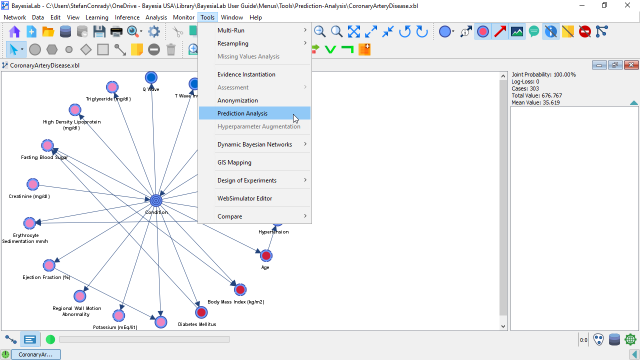
BayesiaLab generates a new model and opens a new Graph Window for it.

Click to Zoom

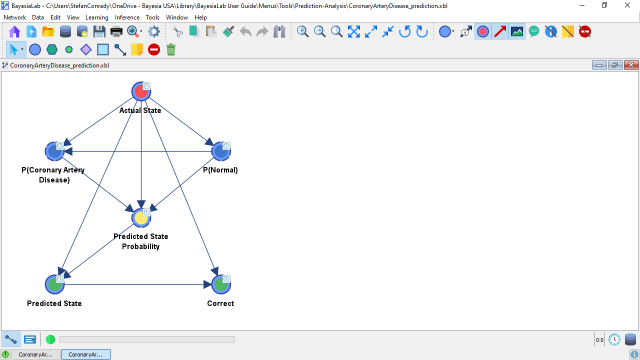
By default, BayesiaLab attaches the suffix “_prediction” to the original file name.

Now, switch to the Validation Mode and bring up all nodes as Monitors in the Monitor Panel.

Click to Zoom

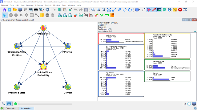
The node $\mathit{Actual\ State}$ represents the ground truth for the Target Node, i.e., the node $\mathit{Condition}$ in the network, which we are analyzing here.

The nodes $P(\mathit{Coronary\ Artery\ Disease})$ and $P(\mathit{Normal})$ show the distributions of the probabilities predicted by the network for each state.

The node $\mathit{Predicted\ State\ Probability}$ represents the probabilities associated with $\mathit{Predicted\ State}$. In other words, it shows the degree of confidence in the prediction. Given that this node represents the probability of the predicted state, the range of probabilities has to be $0.5 < \mathit{Predicted\ State\ Probability} < 1$. A probability below 0.5 would obviously imply that state would not be the predicted one.

The node $\mathit{Predicted\ State}$ is the state the network predicted given the available observations.

Finally, the binary node $\mathit{Correct}$ shows whether $\mathit{Predicted\ State}$ coincides with $\mathit{Actual\ State}$.

Interpretation

The benefit of this model becomes clear once you translate common questions about the performance of a predictive model into queries of the corresponding prediction analysis model.

For instance, we would be interested in how many of the patients who actually had Coronary Artery Disease were predicted as such. So, we set $P(\mathit{Actual\ State}=\mathit{Coronary\ Artery\ Disease})=100\%$.

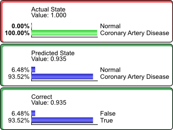
We see that 93.52% of the cases of Coronary Artery Disease were predicted correctly. This value coincides with the Precision value (highlighted by the red border) reported in the Target Analysis Report.

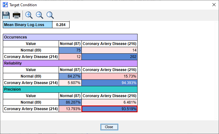
Conversely, we can set $P(\mathit{Predicted\ State}=\mathit{Coronary\ Artery\ Disease})=100\%$.

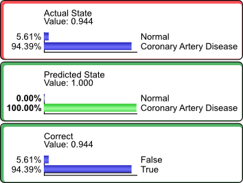
This means that of those patients predicted to have Coronary Artery Disease, 94.39% did actually have the condition. This value coincides with the Reliability value (highlighted by the red border) reported in the Target Analysis Report.

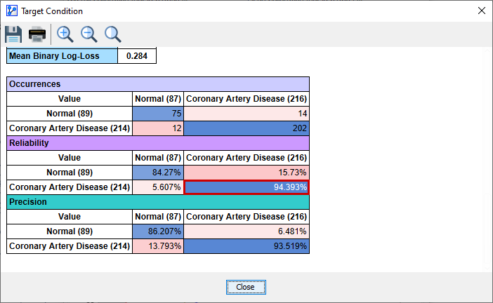
Similarly, any other cell in the Confusion Matrix above can be computed in the same way. Furthermore, we can pursue additional questions that cannot be easily obtained from any report.

For instance, we can examine the distributions that are associated with false predictions, by setting $P(\mathit{Correct}=\mathit{False})=100\%$.

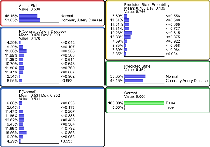
This would suggest that the distribution of false predictions is different from the marginal distribution of the actual state. In certain contexts, it can be valuable to understand the characteristics of false predictions for further refining the model.

Workflow Animation