Target Precision

Context

The Target Precision is one of the measures that can be computed in the Structural Coefficient Analysis and plotted in the Curve window. When plotted, it can help you determine an appropriate value for the Structural Coefficient given your dataset and the learning algorithm you selected. The Target Precision metric is intended to be used primarily in the context of Supervised Learning.

Usage

To illustrate the Target Precision metric, we use a sample network that predicts contraceptive use among married Indonesian women as a function of demographic attributes. This model is based on a subset of variables from the 1987 National Indonesia Contraceptive Prevalence Survey, which is available from the UCI Machine Learning Repository .

HomePricePredictorModel.xbl

XBL

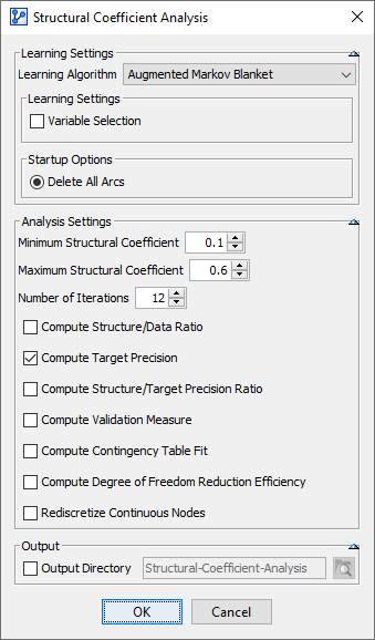
Now, we perform a Structural Coefficient Analysis: Menus > Tools > Multi-Run > Structural Coefficient Analysis. We follow the overall workflow introduced in Structural Coefficient Analysis. Given that this is a predictive model, we select a Supervised Learning algorithm from the settings window. More specifically, we choose the Augmented Markov Blanket and examine a range of 0.05 to 0.5 for the Structural Coefficient in 10 iterations. In the context of a predictive model, the Target Precision is one of the key metrics to evaluate.

Structural Coefficient Analysis settings (Augmented Markov Blanket) for Target Precision

The dataset associated with this model is split into a Learning Set and a Test Set, as indicated by the symbol tagged onto the database icon in the lower right-hand corner of the Graph Window. Given the split, the Structural Coefficient Analysis calculates the Target Precision separately for the Learning Set and the Test Set.

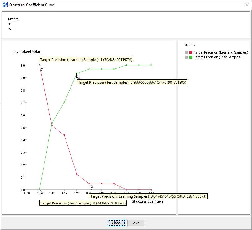
Target Precision curve for the Learning and Test sets

Note that the y-axis is normalized, but you can view the absolute values by hovering over individual points. The values in parentheses are the non-normalized values of Target Precision.

In general, reducing the Structural Coefficient (x-axis) increases the Target Precision (y-axis) for the Learning Samples (red curve). Hence, it is always tempting to decrease the Structural Coefficient in pursuit of higher predictive performance. For SC > 0.25, Target Precision (Learning Samples) appears relatively flat. For $SC < 0.25$ , the Target Precision (Learning Samples) increases very rapidly, potentially suggesting a good predictive performance. However, the performance of the model with regard to the learning set is of little value if it doesn’t hold up in out-of-sample testing.

Indeed, the performance for $SC < 0.25$ does not hold up for the Test Set (green curve). While Target Precision (Test Samples) appears flat for $SC > 0.25$ , it decreases very rapidly for $SC < 0.25$ . In absolute terms, at SC=0.05, the Target Precision (Learning Samples) of 70% is vastly different from the Target Precision (Test Samples) of 45%. This is a very clear sign of overfitting. So, learning with an extremely low value of SC=0.05 would likely produce a model that cannot generalize beyond the learning sample.

As a result, you can use the two curves as an additional visual guide to avoid potential overfitting. Note that this is not a hard-and-fast rule. Rather, you should use this Target Precision plot in the context of all the other available plots.