
Evidence Instantiation
Context
By definition, a Bayesian network represents a Joint Probability Distribution (JPD). Whenever you set any evidence on a network, the JPD becomes smaller, i.e., only a subspace of the original JPD is now represented by the network given the evidence. For many research applications, you may only want to explore that very subspace rather than the JPD as a whole.
Evidence Instantiation provides a way to “extract” the subspace of the JPD as it is defined by the network and the evidence set. It creates a new network that represents only that subspace of the original JPD.
You may think that BayesiaLab achieves this by extracting a subset of the underlying dataset of the original network. However, that is not the case! Rather, the underlying dataset is irrelevant for Evidence Instantiation. Instead, it takes the original network structure and updates its Conditional Probability Tables so that it represents the desired subspace of the original JPD.
Usage & Example
You can perform Evidence Instantiation based on any network that has all Probability Tables and Conditional Probability Tables fully specified or estimated. Note that any type of evidence, including Soft Evidence and Hard Evidence, can be used in the context of Evidence Instantiation. To illustrate Evidence Instantiation, we use the familiar Perfume dataset, which we discuss in Chapter 8: Probabilistic Structural Equation Models of our e-book.

In this example, we focus on the factor nodes, i.e., [Factor_0] through [Factor_7].
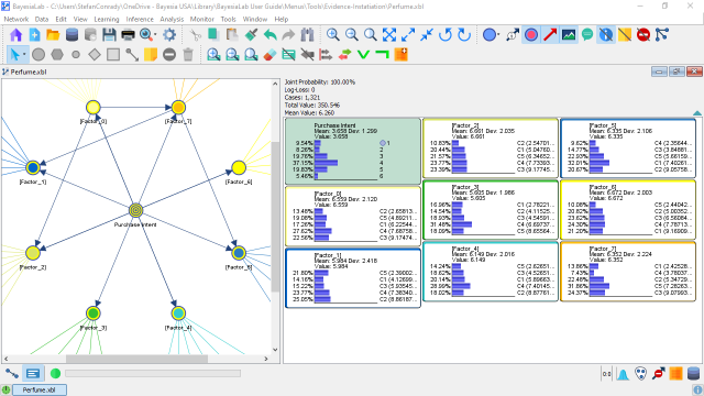
Next, we set an arbitrary set of evidence on the factor nodes. For illustration purposes, we set Numerical Evidence using MinXEnt.
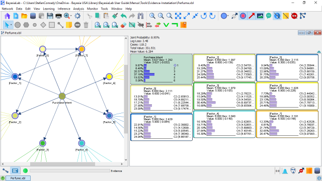
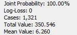
Note the values reported in the Information Panel, right above the Monitor Panel:
- No Evidence Set
- Evidence Set
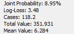
The smaller value of the Joint Probability indicates that we are now looking at a subspace of the original JPD. With this evidence set, we select Menus > Tools > Evidence Instantiation. This brings up a new Graph Window named New Network Instantiation 1.xbl.
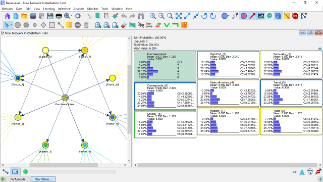
The factor nodes perfectly match the distributions set earlier as evidence. However, these distributions are now marginal distributions, without any evidence set applied. Also, the Information Panel now reports a Joint Probability of 100% again:
- Evidence Set
- Evidence Instantiation
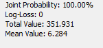
So, the subspace of the original JPD is now the entire JPD of the new network. It is important to know that there is no longer an associated dataset. The Graph Window of the original network featured the database icon to indicate that a dataset is associated with the network. After Evidence Instantiation, the icon is gone. Also, the Information Panel showed the number of cases in the original dataset. With the Evidence Instantiation, the dataset was discarded, so there is no longer any reference to cases. This also means that we would not be able to re-learn the new network, as no data is available for that purpose. However, we can perform inference on the newly instantiated network just like with any other network or the original network.