
Validation Measure
Context
The Validation Measure is available to be plotted within the Curve window as part of the Structural Coefficient Analysis. Formally, the Validation Measure VM is defined as
where LL stands for Log-Loss.
As with all measures provided by the Structural Coefficient Analysis, the Validation Measure supports you in choosing an appropriate value for the Structural Coefficient. The Validation Measure is based on the Log-Loss statistics of the Learning Set and the Test Set. Hence, the associated dataset must already be split into a Learning Set and the Test Set. The Confidence Analysis Report also reports the Validation Measure corresponding to each Comparison Structure.
Usage
To illustrate the use of the Validation Measure, we use a sample network that represents the joint distribution of symptoms related to COVID-19:

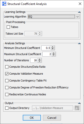
The dataset associated with this model is split into a Learning Set and a Test Set, as indicated by the symbol tagged onto the database icon in the lower right-hand corner of the Graph Window. With this network, we now perform a Structural Coefficient Analysis: Menus > Tools > Multi-Run > Structural Coefficient Analysis. We follow the overall workflow introduced in Structural Coefficient Analysis. Given that the Validation Measure is particularly relevant in the context of Unsupervised Learning, we use EQ as the Learning Algorithm and set a Structural Coefficient range from 0.5 to 2.
Upon clicking the Curve button at the bottom of the report, we obtain the following plot. In the screenshot below, the x-y pairs corresponding to the iterations are shown on the plot:
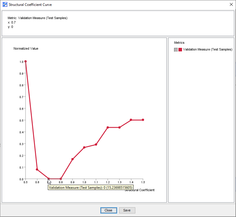
The x-axis represents the Structural Coefficient values, and the y-axis shows the Validation Measure computed for each network learned with the corresponding value of the Structural Coefficient. Note that the y-values are normalized to a 0-to-1 range, i.e., the smallest computed Validation Measure is displayed as 0 and the largest value as 1. Hovering over a point shows the normalized value plus the unnormalized value in parentheses.
Interpretation
The Structural Coefficient values that are associated with the minimum values of the Validation Measure are considered ideal. The u-shaped portion at the bottom of the plotted curve (also referred to as “tub” or “trough”) represents the range of minimum values: . With values of the Structural Coefficient within this approximate range, a model would be neither “overfitted” nor “underfitted.”
Recall the definition of the Validation Measure VM:
where LL stands for Log-Loss.
This means that if the Test Set Log-Loss variance exceeds the Learning Set Log-Loss variance, the Validation Measure increases beyond the Log-Loss of the Test Set. In other words, an optimal Validation Measure can be achieved only if the network’s predictive performance with regard to the Test Set is good, i.e., the Test Set Log-Loss is small, and if the Test Set Log-Loss variance does not exceed the Learning Set Log-Loss variance. Intuitively, this makes sense: if the Test Set Log-Loss variance is greater than the Learning Set Log-Loss variance, the predictive model is not a good generalization of the underlying dataset.