
Data and Import
Exploratory Analysis
Data Overview
In order to better understand the nature of accidents, the National Automotive Sampling System (NASS) Crashworthiness Data System (CDS) was established as a nationwide crash data collection program sponsored by the U.S. Department of Transportation. The National Center for Statistics and Analysis (NCSA), part of the National Highway Traffic Safety Administration (NHTSA), started the data collection for the NASS program in 1979. Data collection is accomplished at 24 geographic sites, called Primary Sampling Units (PSUs). These data are weighted to represent all police-reported motor vehicle crashes occurring in the USA during the year involving passenger cars, light trucks, and vans that were towed due to damage. All data are available publicly from NHTSA’s FTP server.10
Data Set for Study
We use the following subset of files from the 11-file dataset published by NHTSA (ftp://ftp.nhtsa.dot.gov/NASS):
- ACC: Accident Record (accident.sas7bdat)
- GV: General Vehicle Record (gv.sas7bdat)
- OA: Occupant Assessment Record (oa.sas7bdat)
- VE: Exterior Vehicle Record (ve.sas7bdat)
We have joined the records of these tables via their unique identifiers and then concatenated all files from 1995 through 2011 into a single table. This table contains records regarding approximately 200,000 occupants of 100,000 vehicles involved in 37,000 accidents. Each record contains more than 400 variables, although there is a substantial amount of missing values. The comprehensive nature of this dataset is ideal for our exploration of the interactions of crash-related variables and their ultimate impact on passenger safety.
Notation
- All variable names/labels follow the format “DatasetAbbreviation_VariableName”, e.g. GV_SPLIMIT for the variable from the dataset General Vehicle Record.
- All variable and node names are italicized.
- Names of BayesiaLab-specific features and functions are capitalized and shown in bold type.
Data Filters and Variable Selection
To start with our exploration of this problem domain, we narrow our focus by selecting subsets of variables and records:
- We restrict our analysis to horizontal vehicle-to-vehicle collisions, with the vehicle under study being MY2000 or later. We consider MY2000 a reasonable cutoff point, as by then second-generation airbags were mandatory for all passenger vehicles. In this context, we only examine the condition of the driver. Also, we exclude collisions involving large trucks (Gross Vehicle Weight Rating (GVWR) > 10,000 lbs.) and motorcycles. For data consistency purposes, we filter out unusual and very rare accident types, e.g. accidents with principal deformation to the underside of the vehicle. We apply these filters primarily for expositional simplicity. However, we do recognize that this limits our ability to broadly generalize the findings.
- However, no records are excluded solely due to missing values. BayesiaLab offers advanced missing values processing techniques, which we can leverage here. This is an important point as the vast majority of records contain some missing values. In fact, if we applied a traditional casewise/listwise deletion, most records would be eliminated from the database.
- Furthermore, many of the 400+ variables provide a level of detail that far exceeds the scope of this paper. Thus, we limit our initial selection to 19 variables that appear a priori relevant and are generally in line with the variables studied in the EPA/NHTSA research.
- In addition to the variables defined in the NASS/CDS database, we introduce GV_FOOTPRINT as a variable that captures vehicle footprint.13 This new variable is computed as the product of VE_WHEELBAS (Wheelbase) and VE_ORIGAVTW (Average Track Width), which are recorded in the original database (“ is defined as a vehicle’s wheelbase multiplied by its average track width - in other words, the area enclosed by the points at which the wheels meet the ground.” Final Rule, p. 69).
The following table summarizes the variables included in our study.
| Variable Name | Long Name | Units/States | Comment |
|---|---|---|---|
| GV_CURBWGT | Vehicle Curb Weight | kg | |
| GV_DVLAT | Lateral Component of Delta V | km/h | |
| GV_DVLONG | Longitudinal Component of Delta V | km/h | |
| GV_ENERGY | Energy Absorption | J | |
| GV_FOOTPRINT | Vehicle Footprint | m2 | calculated as WHEELBAS x ORIGAVTW |
| GV_LANES | Number of Lanes | count | |
| GV_MODELYR | Vehicle Model Year | year | |
| GV_OTVEHWGT | Weight Of The Other Vehicle | kg | |
| GV_SPLIMIT | Speed Limit | mph | converted into U.S. customary units |
| GV_WGTCDTR | Truck Weight Code | missing = Passenger Vehicle | |
| 6,000 and less | |||
| 6,001-10,000 | |||
| OA_AGE | Age of Occupant | years | |
| OA_BAGDEPLY | Air Bag System Deployed | Nondeployed | |
| Bag Deployed | |||
| OA_HEIGHT | Height of Occupant | cm | |
| OA_MAIS | Maximum Known Occupant AIS | Not Injured | AIS Probability of Death |
| Minor Injury | 0% | ||
| Moderate Injury | 1-2% | ||
| Serious Injury | 8-10% | ||
| Severe Injury | 5-50% | ||
| Critical Injury | 5-50% | ||
| Maximum Injury | 100% (Unsurvivable) | ||
| Unknown | Missing Value | ||
| OA_MANUSE | Manual Belt System Use | Used | |
| Not Used | |||
| OA_SEX | Occupant’s Sex | Male | |
| Female | |||
| OA_WEIGHT | Occupant’s Weight | kg | |
| VE_GAD1 | Deformation Location (Highest) | Left | |
| Front | |||
| Rear | |||
| Right | |||
| VE_PDOF_TR | Clock Direction for Principal Direction of Force (Highest) | Degrees | Transformed variable, rotated 135 degrees counterclockwise |
OA_MAIS (Maximum Known Occupant AIS)
The outcome variable represents the . “AIS” stands for “Abbreviated Injury Scale.” The Abbreviated Injury Scale is an anatomically-based, consensus-derived global severity scoring system that classifies each injury by body region according to its relative importance on a 6-point ordinal scale (1=minor and 6=maximal).
Coordinate System for Variable PDOF1 (Principal Direction of Force)
Most of the variables’ scales and units are self-explanatory, perhaps with the exception of GV_PDOF1 (Principal Direction of Force). This variable records the direction of the highest force acting on the vehicle during the accident. A frontal collision, i.e. in the direction of travel from the perspective of the vehicle under study, would imply PDOF1=0. Conversely, a rear impact would mean PDOF1=180, etc.
Given the requirements of data discretization as part of the data import process (see next chapter), we rotate the coordinate system by 135 degrees counterclockwise. The values in this new coordinate system are recorded in the transformed variable . This rotation prevents that frequently occurring, similar values (e.g. frontal collisions at 355 degrees, 0 degrees, and 5 degrees on the original scale) are split into different bins due to the natural break at 0 degrees.
To make it easier to interpret the values of the transformed variable , we briefly illustrate our new coordinate system. For instance, a VE_PDOF_TR=45 now means that the vehicle under study collided on the driver’s side and that the impact was perpendicular to the direction of travel. A 135 degrees impact represents a direct frontal collision, e.g. with oncoming traffic. Conversely, a rear-end collision is represented by a 315 degrees angle.
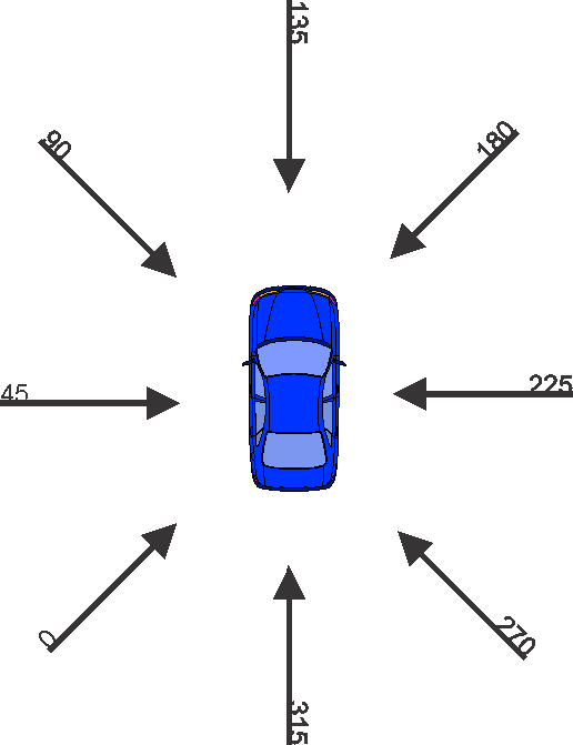
This coordinate system may become more intuitive to understand when it is viewed in quadrant form, in a clockwise direction:
- 0 degrees-90 degrees: Impact from left
- 90 degrees-180 degrees: Frontal impact
- 180 degrees-270 degrees: Impact from right
- 270 degrees-360 degrees: Rear impact
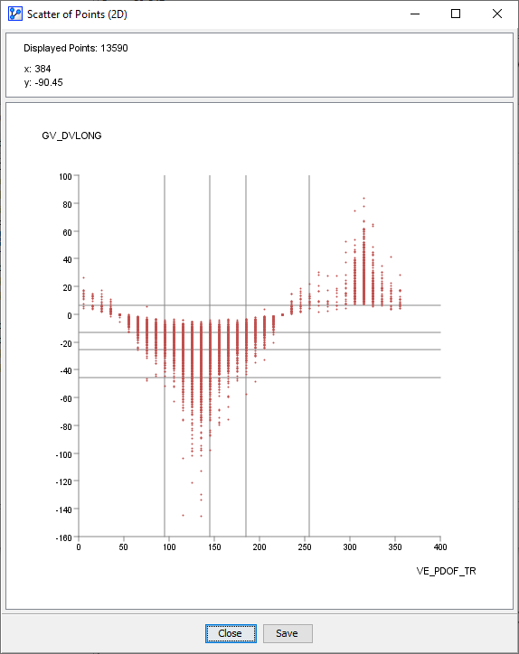
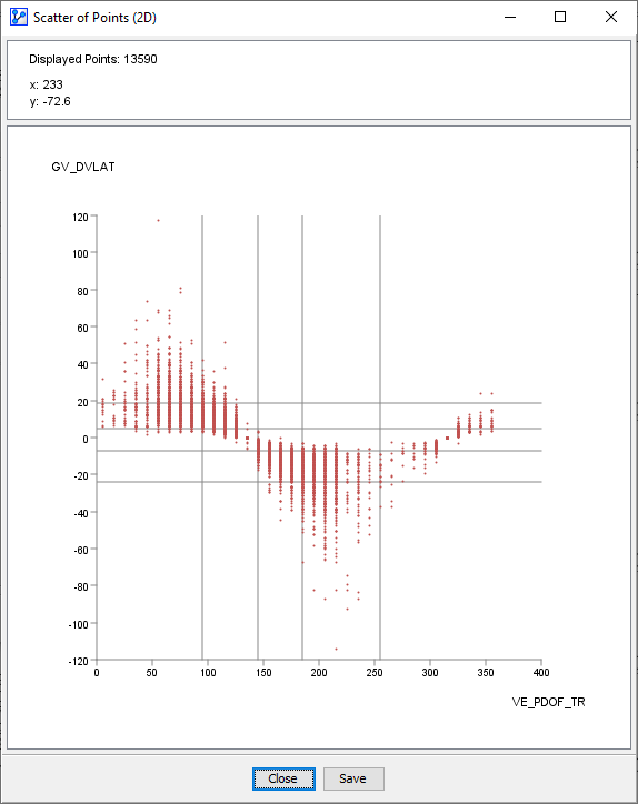
To confirm the plausibility of this transformed variable, we can plot GV_DVLAT and GV_DVLONG as a function of . We would anticipate that a full frontal impact, i.e. _VE_PDOF_TR=135, would be associated with the highest decrease in velocity, i.e. GV_DVLONG≪0. At the same time, we would expect the lateral Delta V to be near zero, i.e. GV_DVLAT≈0. This is indeed what the following plots confirm. They also illustrate the respective signs of Delta V as a function of the impact angle.
In BayesiaLab, we can quickly create scatterplots by selecting Menus > Data > Charts.
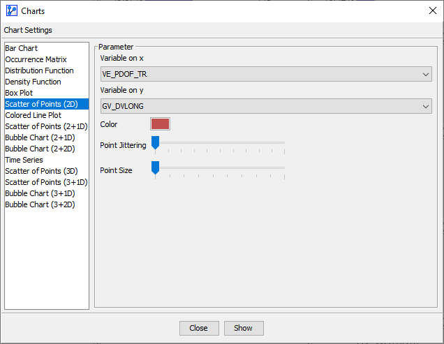
Upon selecting the respective variables for display, BayesiaLab produces the corresponding plots.
Data Import
The first step in our process towards creating a Bayesian network is importing the raw data into BayesiaLab. Please see Open Data Source (Data Import Wizard) for details of the data import workflow.
However, we should note that we adjust some of the bins that were found by BayesiaLab’s automatic discretization algorithms, so they reflect typical conventions regarding this domain. For instance, if the discretization algorithm proposed a bin threshold of 54.5 for GV_SPLIMIT, we would change this threshold to 55 (mph) in order to be consistent with our common understanding of speed limits.
Upon completion of the import process, we obtain an initially unconnected network, which is shown below. All variables are now represented by nodes, one of the core building blocks in a Bayesian network. A node can stand for any variable of interest. Discretized nodes are shown with a dashed outline, whereas solid outlines indicate discrete variables, i.e. variables with either categorical or discrete numerical values. Once the variables appear in this new form in a graph, we will exclusively refer to them as nodes.
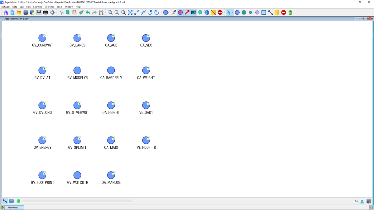
At this point, it is practical to add Long Node Names to the Node Names that are displayed under each node by default. In BayesiaLab, Long Node Names are typically used for more descriptive titles, which can be turned on or off, depending on the desired view of the graph. Here, we associate a dictionary with Long Node Names, while the more compact variable names of the original dataset remain as Node Names (to maintain a compact presentation, we will typically use the original variable name when referencing a particular node).
The syntax for this association is rather straightforward: we simply define a text file that includes one Node Name per line. Each Node Name is followed by the equal sign (“=”), or alternatively TAB or SPACE, and then by the long variable description, which will serve as the Long Node Name.
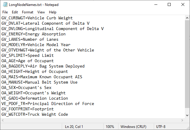
This file can then be loaded into BayesiaLab via Menus > Data > Associate Dictionary > Node > Long Names. Then, after highlighting all nodes, we can select Node Contextual Menu > Properties > Rendering Properties > Show Long Name. Checking the Show Long Name box and clicking OK, brings up the Long Names in the Graph Panel.
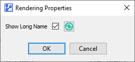
Long Node Names can be displayed either for all nodes or only for selected ones. Given the sometimes cryptic nature of the original variable names, we will keep the more self-explanatory Long Node Names turned on for most analyses. Also, we can separately turn on the Long Names for the Monitor Panel: Monitor Panel Contextual Menu > Show > Long Name of Nodes.