Modeling Injury Severity with Supervised Learning

While Unsupervised Learning is an ideal way to examine multiple interactions within our domain for exploratory purposes, the principal task at hand is explaining injury severity ($\mathit{Maximum\ Known\ Occupant\ AIS}$) as a function of the other variables. The Monitor for $\mathit{Maximum\ Known\ Occupant\ AIS}$ reminds us of the marginal distribution of this variable, which shall serve as a reference point for subsequent comparisons.

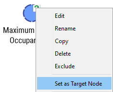
BayesiaLab offers a number of Supervised Learning algorithms that allow us to focus on a target variable. We set $\mathit{Maximum\ Known\ Occupant\ AIS}$ as the Target Node via the node’s Contextual Menu, thus defining it as the principal variable of interest.

Furthermore, we designate $\mathit{Maximum\ Known\ Occupant\ AIS}=\mathrm{4-6}$ as the Target State of the Target Node, which will subsequently allow us to perform certain analyses with regard to this particular state, i.e. the most serious injuries.

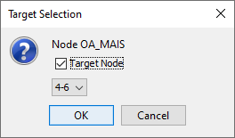
Note that pressing T, while double-clicking a state within a Monitor, also allows setting the Target Node and the Target State.

Augmented Naive Bayes Learning

Now that the Target Node is defined, we have an array of Supervised Learning algorithms available. Given the small number of nodes, variable selection is not an issue and hence this should not influence our choice of algorithm. Furthermore, the number of observations does not create a challenge in terms of computational effort. With these considerations, and without going into further detail, we select the Augmented Naive Bayes algorithm. “Naive” refers to a network structure in which the Target Node is connected directly to all other nodes. Such a Naive Bayes structure is generated by specification, rather than by machine learning. The “augmented” part in the name of this algorithm refers to the additional unsupervised search that is performed on the basis of the given naive structure.

We start the learning process from the menu by selecting Menus > Learning > Supervised Learning > Augmented Naive Bayes. Upon completion of the learning process, we apply the Automatic Layout algorithm P, and BayesiaLab presents the following new network structure.

The predefined Naive Bayes structure is highlighted with the dotted arcs, while the augmented arcs (from the additional Unsupervised Learning) are shown with solid arcs.

Once the network is learned, bringing up the Mapping function and selecting Pearson Correlation for the Arc Analysis provides an instant survey of the dynamics in the network.

Click to Zoom

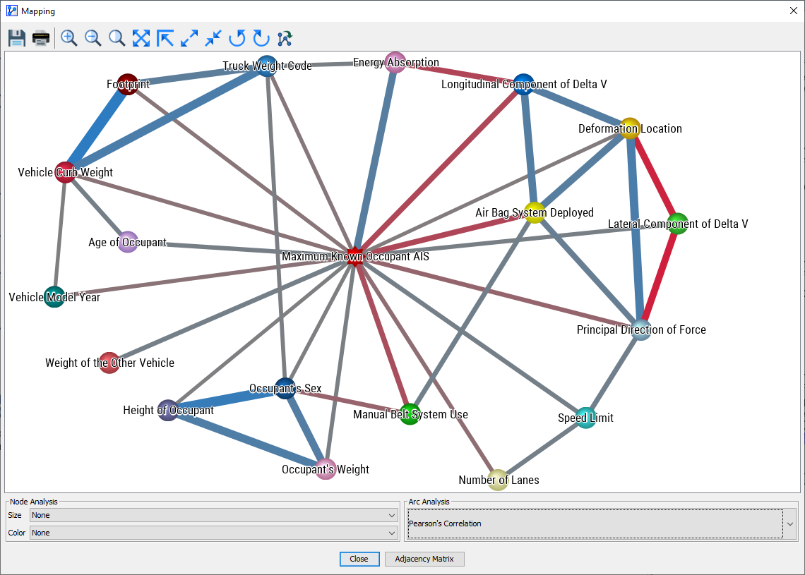
As always, the caveat applies that Pearson Correlation should only be interpreted as such if the assumption of linearity can be made.

Structural Coefficient Analysis

Even if we find everything to be reasonable, we will need to ask the question of whether this model does include all important interactions. Did we learn a reliable model that can be generalized? Is the model we built the best one among all the possible networks? Is the model possibly overfitted to the data?

Some of these questions can be studied with BayesiaLab’s Structural Coefficient Analysis. Before we delve into this function, we first need to explain the Structural Coefficient (SC). It is a kind of significance threshold that can be adjusted by the analyst and that influences the degree of complexity of the induced network.

By default, this Structural Coefficient is set to 1, which reliably prevents the learning algorithms from overfitting the model to the data. In studies with relatively few observations, the analyst’s judgment is needed for determining a possible downward adjustment of this parameter. On the other hand, when data sets are large, increasing the parameter to values greater than 1 will help manage the network complexity.

BayesiaLab can systematically examine the question of optimal complexity with the Structural Coefficient Analysis. In our example, we wish to know whether a more complex network, while avoiding overfit, would better capture the dynamics of our domain. Structural Coefficient Analysis generates several metrics that can help in making this trade-off between complexity and fit: Menus > Tools > Multi-Run > Structural Coefficient Analysis.

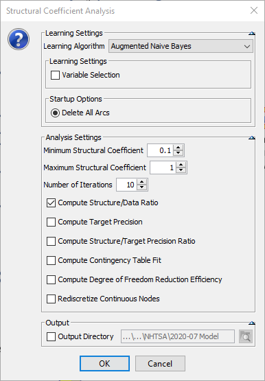
BayesiaLab prompts us to specify the range of the Structural Coefficient to be examined and the number of iterations to be performed. It is worth noting that the Minimum Structural Coefficient should not be set to 0, or even close to 0. A value of 0 would lead to learning a fully connected network, which can take a long time depending on the number of variables, or even exceed the memory capacity of the computer running BayesiaLab.

The Number of Iterations determines the steps to be taken within the specified range of the Structural Coefficient. We leave this setting at the default level of 10. For metrics, we select Compute Structure/Data Ratio, which we will subsequently plot.

The resulting report shows how the network changes as a function of the Structural Coefficient. For other analyses based on Cross-Validation, this report can be used to determine the degree of confidence we should have in any particular arc in the structure.

Our overall objective here is to determine the correct level of network complexity for representing the interactions with the Target Node without the overfitting of data. By clicking Curve we can plot the Structure/Data Ratio (y-axis) over the Structural Coefficient (x-axis).

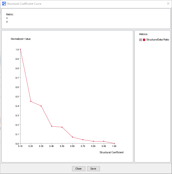
Typically, the “elbow” of the L-shaped curve above identifies a suitable value for the Structural Coefficient (SC). The visual inspection suggests that an SC value of around 0.35 would be a good candidate. Further to the left of this point, e.g. SC≈0.1, the complexity of the model increases much more than the likelihood of the data given the model. This means that arcs would be added without any significant gain in terms of better representing the data. That is the characteristic pattern of overfitting, which is what we want to avoid.

Given the results from this Structural Coefficient Analysis, we can now relearn the network with an SC value of 0.35. The SC value can be set via Graph Panel Contextual Menu > Edit Structural Coefficient or Menus > Edit > Edit Structural Coefficient.

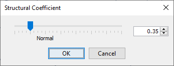
Once we relearn the network, using the same Augmented Naive Bayes algorithm as before, we obtain a more complex network.

Example 2: Seat Belt Usage

Similar to the analysis we performed earlier on $\mathit{Number\ of\ Lanes}$, $\mathit{Speed\ Limit}$, and $\mathit{Deformation\ Location}$, we will now examine the Target Node, $\mathit{Maximum\ Known\ Occupant\ AIS}$. We select and double-click the nodes $\mathit{Maximum\ Known\ Occupant\ AIS}$ and $\mathit{Manual\ Belt\ System\ Use}$ to bring them up in the Monitor Panel.

Initially, the Monitors show $\mathit{Maximum\ Known\ Occupant\ AIS}$ and $\mathit{Manual\ Belt\ System\ Use}$ with their marginal distributions (1st column from left). We now set evidence on $\mathit{Manual\ Belt\ System\ Use}$ to evaluate the changes to $\mathit{Maximum\ Known\ Occupant\ AIS}$. Our experience tells us that not wearing a seatbelt is associated with an increased risk of injury in an accident.

Indeed, this is precisely what we observe. For example, for $\mathit{Manual\ Belt\ System\ Use}=\mathrm{Not\ Used}$ the probability of no/minor injury is 66.87% (2nd column). On the other end of the injury spectrum, the probability of serious injuries is 8.21%.

The situation is much better for $\mathit{Manual\ Belt\ System\ Use}=\mathrm{Used}$ (3rd column). The probability of no/minor injury is higher (+19.2 percentage points), and the probability of serious injury is much lower (-5.7 percentage points). These results appear intuitive and are in sync with our domain knowledge.

However, does this confirm that wearing a seat belt reduces the risk of sustaining a serious injury by roughly two-thirds? Not yet.

We can further examine this by including the variable $\mathit{Air\ Bag\ System\ Deployed}$. The bottom-left Monitor shows the marginal distribution of $\mathit{Air\ Bag\ System\ Deployed}$.

To compare the conditions $\mathit{Manual\ Belt\ System\ Use}=\mathrm{Not\ Used}$ and $\mathit{Manual\ Belt\ System\ Use}=\mathrm{Used}$, we first set evidence on $\mathrm{Not\ Used}$ (2nd column, 2nd row). The posterior distribution of $\mathit{Maximum\ Known\ Occupant\ AIS}$ has an expected value of 1.341, and the probability of $\mathit{Air\ Bag\ System\ Deployed}=\mathrm{Deployed}$ has increased to 63.71%. Because $\mathit{Maximum\ Known\ Occupant\ AIS}$ has an ordinal rather than numerical scale, we need to be careful when interpreting its expected values (means).

Setting the evidence $\mathit{Manual\ Belt\ System\ Use}=\mathrm{Used}$ (3rd column, 2nd row) changes the expected value of $\mathit{Maximum\ Known\ Occupant\ AIS}$ to 0.860, a decrease of 0.481, but it is also associated with a much different posterior distribution of $\mathit{Air\ Bag\ System\ Deployed}$, which now has a lower probability for Deployed. How should we interpret this?

As it turns out, many airbag systems are designed in such a way that their deployment threshold is adjusted when occupants are not wearing seat belts (Bosch Automotive Handbook, 2011, p. 933). This means that not wearing a seat belt causes the airbag to be triggered differently. So, beyond the direct effect of the seat belt, whether or not it is worn indirectly influences the injury risk via the trigger mechanism of the airbag system.

Covariate Imbalance

Beyond the link between seat belt and airbag, there are numerous other relevant relationships. For instance, seat belt users are more likely to be female, they are older and they are, for some unknown reason, less likely to be involved in a frontal crash, etc.

Similar to the earlier example, the evidence set on $\mathit{Manual\ Belt\ System\ Use}$ is propagated omnidirectionally through the network, and the posterior distributions of all nodes are updated. The Monitors below show the difference between the evidence $\mathit{Manual\ Belt\ System\ Use}=\mathrm{Not\ Used}$ (left set of panels) and $\mathit{Manual\ Belt\ System\ Use}=\mathrm{Used}$ (right).

This highlights that seat belt users and non-users are quite different in their characteristics and thus not directly comparable. So, what is the benefit of the seat belt, if any?

In fact, this is a prototypical example of the challenges associated with observational studies. By default, observational studies, like the one here, permit only observational inference. However, performing observational inference on $\mathit{Maximum\ Known\ Occupant\ AIS}$ given $\mathit{Manual\ Belt\ System\ Use}$ is of limited use for the researcher or the policymaker. How can we estimate causal effects with observational data? How can we estimate the (hopefully) positive effect of the seat belt?

Within a traditional statistical framework, a number of approaches would be available to address such differences in characteristics, including stratification, adjustment by regression, and covariate matching (e.g. Propensity Score Matching). For this tutorial, we will proceed with a method that is similar to covariate matching; however, we will do this within the framework of Bayesian networks.

Likelihood Matching with BayesiaLab

We will now briefly introduce the Likelihood Matching (LM) algorithm, which was originally implemented in the BayesiaLab software package for “fixing” probability distributions of an arbitrary set of variables, thus allowing us to easily define complex sets of soft evidence. The Likelihood Matching algorithm searches for a set of likelihood distributions, which, when applied on the Joint Probability Distribution (JPD) encoded by the Bayesian network, allows obtaining the posterior probability distributions defined (as constraints) by the user.

This allows us to perform matching across all covariates while taking into account all their interactions, and thus to estimate the direct effect of $\mathit{Manual\ Belt\ System\ Use}$. We will now illustrate a manual approach for estimating the effect; in the next chapter, we will show a more automated approach with the Direct Effects function.

Fixing Distributions

We start with the marginal distributions of all nodes. Next, we select all covariate nodes in the Monitor Panel and then select Monitor Contextual Menu > Fix Probabilities.

Click to Zoom

This “fixes” the (marginal) distributions of these covariate nodes. Their new fixed condition is indicated by the purple color of the bars in the Monitors.

If we now set the evidence on $\mathit{Manual\ Belt\ System\ Use}=\mathrm{Used}$, we will see no significant changes in these fixed covariate distributions. The Likelihood Matching algorithm has indeed obtained materially equivalent distributions.

Causal Inference

Given that the covariate distributions remain fixed, we can now exclusively focus on the Target Node $\mathit{Maximum\ Known\ Occupant\ AIS}$:

$\mathit{Manual\ Belt\ System\ Use}=\mathrm{Not\ Used}$

$\mathit{Manual\ Belt\ System\ Use}=\mathrm{Used}$

If we make the assumption that no other unobserved confounders exist in this domain, we will now be able to give the change in the distribution of $\mathit{Maximum\ Known\ Occupant\ AIS}$ a causal interpretation. This would represent the difference between forcing all drivers to wear a seat belt versus forcing all of them not to do so.

More formally we can express such an intervention with Pearl’s do-operator, which reflects actively setting of a condition (or intervention) versus merely observing a condition:

Observational Inference:

In words: the probability of $\mathit{Maximum\ Known\ Occupant\ AIS}$ taking on the value $\mathrm{4-6}$ given (“|”) that $\mathit{Manual\ Belt\ System\ Use}$ is observed as $\mathrm{Used}$.

$P(Maximum Known Occupant AIS=4-6 \mid Manual Belt System Use=Used)=2.55\%$

P($\mathit{Maximum\ Known\ Occupant\ AIS}=\mathrm{4-6}$|$\mathit{Manual\ Belt\ System\ Use}=\mathrm{Not\ Used}$)=8.21%

Causal Inference:

In words: the probability of $\mathit{Maximum\ Known\ Occupant\ AIS}$ taking on the value $\mathrm{4-6}$ given (“|”) that $\mathit{Manual\ Belt\ System\ Use}$ is actively set (by intervention) to “Used.”

P($\mathit{Maximum\ Known\ Occupant\ AIS}=\mathrm{4-6}$|do($\mathit{Manual\ Belt\ System\ Use}=\mathrm{Used}$))=2.71%

P($\mathit{Maximum\ Known\ Occupant\ AIS}=\mathrm{4-6}$|do($\mathit{Manual\ Belt\ System\ Use}=\mathrm{Not\ Used}$))=5.99%

From these results we can easily calculate the causal effect:

P($\mathit{Maximum\ Known\ Occupant\ AIS}=\mathrm{4-6}$|do($\mathit{Manual\ Belt\ System\ Use}=\mathrm{Used}$)) - P($\mathit{Maximum\ Known\ Occupant\ AIS}=\mathrm{4-6}$|do($\mathit{Manual\ Belt\ System\ Use}=\mathrm{Not\ Used}$)) = -3.28%

We conclude that this difference, -3.28 percentage points, is the “seat belt effect” with regard to the probability of serious injury. Analogously, the effect for moderate injuries is -10.14 percentage points. Finally, for no/minor injuries, there is a positive effect of 13.4 percentage points.

With “causal inference” formally established and implemented through this workflow, we can advance to the principal question of this study, the influence of vehicle size and weight on injury risk.