Effect of Weight and Size on Injury Risk

Our previous example regarding seat belt usage illustrated the challenges of estimating causal effects from observational data. It became clear that the interactions between variables play a crucial role. Furthermore, we have shown how Likelihood Matching, under the assumption of no unobserved covariates, allows us to estimate the causal effect from observational data.

Lack of Covariate Overlap

Before we continue with the effect estimation of vehicle weight and size, we will briefly review the distributions of the nodes under study, $\mathit{Vehicle\ Curb\ Weight}$, and $\mathit{Footprint}$ as a function of $\mathit{Truck\ Weight\ Code}$. We can use this code to select classes of vehicles, including Passenger Car, Truck < 6,000 lbs., and Truck < 10,000 lbs.

We can see that the distributions of $\mathit{Vehicle\ Curb\ Weight}$ and $\mathit{Footprint}$ are very different between these vehicles’ classes. For $\mathit{Truck\ Weight\ Code}=\mathrm{Passenger\ Car}$, we have virtually no observations in the two highest bins of $\mathit{Vehicle\ Curb\ Weight}$ (left column), whereas for large trucks ($\mathit{Truck\ Weight\ Code}=\mathrm{Truck}$ < 10,000 lbs.) the two bottom bins are almost empty (right column). We see a similar situation for $\mathit{Footprint}$.

This poses two problems: Firstly, we now have a rather “coarse” discretization of values within each class of vehicles, which could potentially interfere with estimating the impact of small changes in these variables. Secondly, and perhaps more importantly, the lack of covariate overlap may prevent the Likelihood Matching algorithm from converging on matching likelihoods between variables. As a result, we might not be able to carry out any causal inference. Hence, we must digress for a moment and resolve this issue in the following section on Multi-Quadrant Analysis.

Multi-Quadrant Analysis

BayesiaLab offers a way to conveniently overcome this fairly typical problem. We can perform a Multi-Quadrant Analysis that will automatically generate a Bayesian network for each vehicle subset, i.e. Passenger Car, Truck < 6,000 lbs., and Truck < 10,000 lbs.

The Multi-Quadrant Analysis can be started via Menus > Analysis > Visual > Segment > Multi-Quadrant.

We now need to set several options: The Breakout Variable (or selector variable) must be set to $\mathit{Truck\ Weight\ Code}$, so we will obtain one network for each state of this node. By checking Regenerate Values, the values of each state of each (continuous) node are re-computed from the data of each subset database, as defined by the Breakout Variable. Rediscretize Continuous Nodes is also an option in this context, but we will defer this step and later perform the re-discretization manually. Finally, we set an output directory where the newly generated networks will be saved.

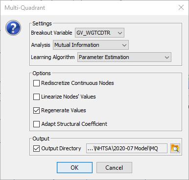
Upon completion of this step, BayesiaLab presents a set of plots, one for each state of the Breakout Variable, $\mathit{Truck\ Weight\ Code}$.

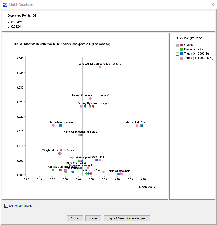
These plots allow us to compare the Mutual Information of each node in the network with regard to the Target Node, $\mathit{Maximum\ Known\ Occupant\ AIS}$. These plots can be very helpful in determining the importance of individual variables in the context of their respective subset.

In our example, we will omit to go into further detail here and instead inspect the newly generated networks. We can simply open them directly from the previously specified location. The new file names follow this format: original filename & “_MULTI_QUADRANT_” & Breakout Variable State & “.xbl”

Vehicle Class: Passenger Car

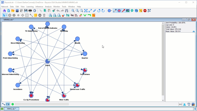
When opening the Passenger Car file, we will notice that the structure is exactly the same as in the network that applied to the whole set. However, examining the Monitors will reveal that the computed probabilities now apply to the Passenger Car subset only.

Since $\mathit{Truck\ Weight\ Code}$ now only contains a single state at 100%, i.e. the same for each record in the Passenger Car subset, we can go ahead and remove this node from the network. We first select the node and then hit the delete key.

Now we can focus our attention on the two variables that prompted the Multi-Quadrant Analysis, namely $\mathit{Vehicle\ Curb\ Weight}$ and $\mathit{Footprint}$. By double-clicking on $\mathit{Vehicle\ Curb\ Weight}$ we bring up the Node Editor, which allows us to review and adjust the discretization of this particular node.

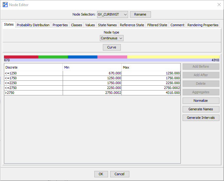
We could directly change the thresholds of the bins in this table. However, it is helpful to bring up the Density Function after clicking on Curve.

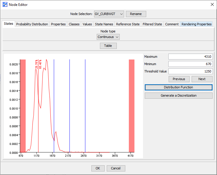
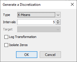
We can now use one of BayesiaLab’s discretization algorithms to establish new bins that are more suitable for the distribution of $\mathit{Vehicle\ Curb\ Weight}$ within the Passenger Car subset. Here, we will use the K-Means algorithm with five intervals.

Upon discretization, the new bin intervals are highlighted in an updated PDF plot.

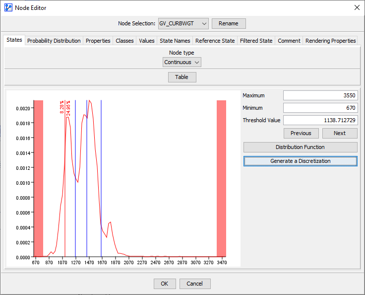
Instead of automatically determining the bins, we could also manually specify them. In our case, we take the bins proposed by the K-Means algorithm and round them to the nearest 50 kg:

We apply the same approach for $\mathit{Footprint}$ and present the result in the following Monitor.

Both discretizations now adequately capture the underlying distributions of the respective variables within the subset Passenger Car.

We now proceed to our principal question of how $\mathit{Vehicle\ Curb\ Weight}$ and $\mathit{Footprint}$ affect $\mathit{Maximum\ Known\ Occupant\ AIS}$. It might be tempting to immediately apply the same process as with the seat belt effect estimation, i.e. fix all covariates with Likelihood Matching and then simulate the response of $\mathit{Maximum\ Known\ Occupant\ AIS}$ as a function of changing values of $\mathit{Vehicle\ Curb\ Weight}$ and $\mathit{Footprint}$. Indeed, we wish to keep everything else the same in order to determine the exclusive Direct Effects of $\mathit{Vehicle\ Curb\ Weight}$ and $\mathit{Footprint}$ on $\mathit{Maximum\ Known\ Occupant\ AIS}$.

However, fixing must not apply to all nodes. Following the definition of kinetic energy,

$\mathit{Energy\ Absorption}$ is a function of $\mathit{Vehicle\ Curb\ Weight}$, $\mathit{Longitudinal\ Component\ of\ Delta\ V}$, and $\mathit{Lateral\ Component\ of\ Delta\ V}$.

This means that $\mathit{Energy\ Absorption}$ cannot be maintained at a fixed distribution as we test varying values of $\mathit{Vehicle\ Curb\ Weight}$ and $\mathit{Footprint}$.

It is important to understand that the relationship of $\mathit{Vehicle\ Curb\ Weight}$ versus $\mathit{Energy\ Absorption}$ is different from, for instance, $\mathit{Vehicle\ Curb\ Weight}$ versus $\mathit{Longitudinal\ Component\ of\ Delta\ V}$ or $\mathit{Lateral\ Component\ of\ Delta\ V}$. The node $\mathit{Energy\ Absorption}$ must be allowed to “respond” in our simulation, as in observational inference, while $\mathit{Longitudinal\ Component\ of\ Delta\ V}$ or $\mathit{Lateral\ Component\ of\ Delta\ V}$ have to be kept at a fixed distribution.

Non-Confounders

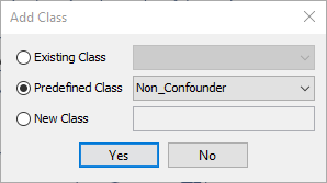
BayesiaLab offers a convenient way to address this requirement. We can assign a special pre-defined Class to variables like $\mathit{Energy\ Absorption}$, called Non_Confounder. We can assign a Class by right-clicking the node $\mathit{Energy\ Absorption}$ and selecting Properties > Classes > Add from the Contextual Menu.

Now, we select the Predefined Class Non_Confounder from the drop-down menu.

The Class icon in the bottom right corner of the screen indicates that a Class has been set.

Direct Effects

The principal question of this study now adds one further challenge in that we are looking for the effect of a continuous variable, $\mathit{Vehicle\ Curb\ Weight}$, as opposed to the effect of a binary variable, such as $\mathit{Manual\ Belt\ System\ Use}$. This means that our Likelihood Matching algorithm must now find matching confounder distributions for a range of values of $\mathit{Vehicle\ Curb\ Weight}$ and $\mathit{Footprint}$.

As opposed to manually fixing distributions via the Monitors, we now use BayesiaLab’s Direct Effects function that performs this automatically. Thus, all Confounder nodes will be fixed in their distributions, excluding the nodes currently being manipulated, the Target Node, and the Non-Confounder nodes.

Although we are primarily interested in the effect of $\mathit{Vehicle\ Curb\ Weight}$ and $\mathit{Footprint}$ on $\mathit{Maximum\ Known\ Occupant\ AIS}$, we will also consider another weight-related node, i.e. Weight of the Other Vehicle, which represents the curb weight of the other vehicle involved in the collision. Given the principle of conservation of linear momentum, we would expect that, everything else being equal, increasing the weight of one’s own vehicle would decrease injury risk, while an increase in the weight of the collision partner would increase injury risk.

We can select these three nodes in the network and then perform a Target Mean Analysis by Direct Effect by selecting Analysis > Visual > Target > Target's Posterior > Curves > Direct Effects.

Given that only a subset of nodes was selected, we are prompted to confirm this set of three nodes.

In our case, we have different types of variables, e.g. $\mathit{Footprint}$, measured in m2, and $\mathit{Vehicle\ Curb\ Weight}$ and Weight of the Other Vehicle, measured in kg. As such, they could not be properly presented in a single plot, unless their x-ranges were normalized. Thus, it is helpful to select Normalize from the options window.

Click to Zoom

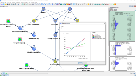
Once this is selected, we can continue to Display Sensitivity Chart.

Click to Zoom

The Direct Effects curves of $\mathit{Vehicle\ Curb\ Weight}$ and Weight of the Other Vehicle have the expected slope. However, $\mathit{Footprint}$ appears “flat,” which is somewhat counterintuitive.

Alternatively, we can exclusively focus on $\mathit{Vehicle\ Curb\ Weight}$ and Weight of the Other Vehicle, which allows us to look at them on their original scales in kilograms. Thus, we select Mean instead of Normalize as the display option.

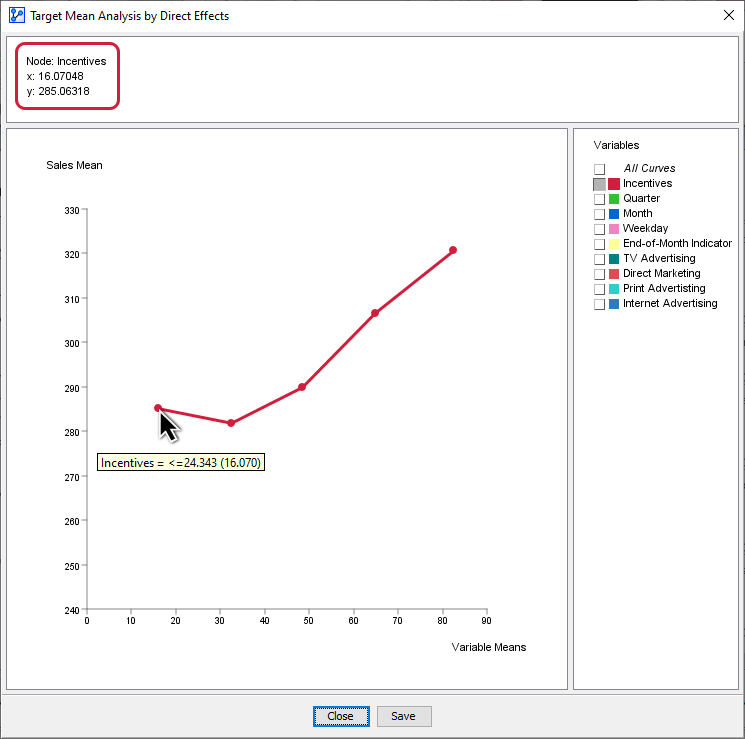
Note that the $\mathit{Vehicle\ Curb\ Weight}$ range is smaller than that of Weight of the Other Vehicle, which was not apparent on the normalized scale. With the Multi-Quadrant Analysis, we had previously generated specific networks for each vehicle class. As a result, the range of $\mathit{Vehicle\ Curb\ Weight}$ in each network’s database is delimited by the maximum and minimum values of each vehicle class. Furthermore, the maximum and minimum values that can be simulated within each network are constrained by the highest and lowest values that the states of the node $\mathit{Vehicle\ Curb\ Weight}$ can represent. We can easily see these limits in the Monitors.

For Passenger Car, $\mathit{Vehicle\ Curb\ Weight}$ ∈ [1133.912, 1807.521]. This also means that we cannot simulate outside this interval and are thus unable to make a statement about the shape of the Direct Effects curves outside these boundaries.

However, within this interval, the simulated Direct Effects curves confirm our a priori beliefs based on the laws of physics regarding the effects of vehicle mass. As both curves appear fairly linear, it is reasonable to have BayesiaLab estimate the slope of the curves around their mean values. We do this by selecting Menus > Analysis > Report > Target > Direct Effects on Target.

A results window shows the estimated Direct Effects in table format.

These Direct Effects can be interpreted similarly to coefficients in a regression. This means that increasing $\mathit{Vehicle\ Curb\ Weight}$ by 100 kg would bring about a 0.02 decrease in the expected value of $\mathit{Maximum\ Known\ Occupant\ AIS}$. On a 0-6 scale, this may seem like a minute change.

However, a negligible change in the expected value (or mean) can “hide” a substantial change in the distribution of $\mathit{Maximum\ Known\ Occupant\ AIS}$, which is illustrated below. An increase of 0.02 in the expected value translates into an 8% (or 0.3 percentage points) increase in the probability of a serious or fatal injury.

Click to Zoom

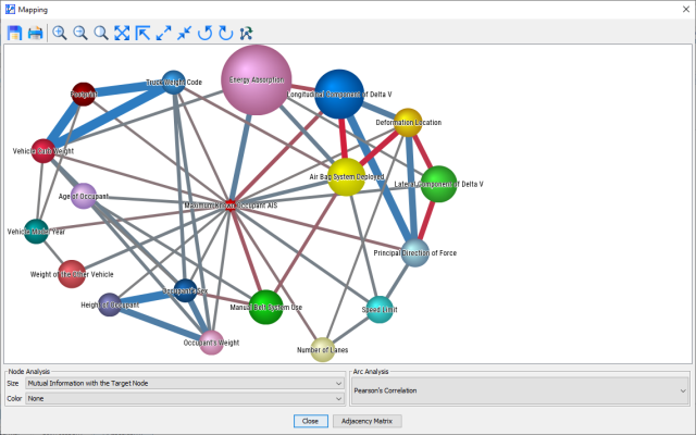
In the example, the changes in the probability of serious injury are in the order of magnitude of one-tenth of one percent. These numbers may appear minute, but they become fairly substantial when considering that roughly 10 million motor vehicle accidents occur in the United States every year. For instance, an increase of 0.1 percentage points in the probability of serious injury would translate into 10,000 human lives that are profoundly affected.

Entire Vehicle Fleet

At the beginning of this section on effect estimation, we made a case for Multi-Quadrant Analysis due to a lack of complete covariate overlap. Consequently, we could only estimate the effects of size and weight by vehicle class. However, the big picture remains of interest. What do these effects look like across all vehicle classes? Despite our initial concerns regarding the lack of overlap, would it perhaps be possible to “zoom-out” to assess these dynamics for the entire vehicle fleet? We will now attempt to do just that and perform inference at the fleet level. There is, unfortunately, no hard-and-fast rule that tells us in advance what amount of overlap is sufficient to perform inference correctly. However, BayesiaLab contains a built-in safeguard and alerts us when Likelihood Matching is not possible.

Keeping the above caveats in mind, we return to our original network, i.e. the one we had learned before applying the Multi-Quadrant Analysis. We now wish to see whether the class-specific effects are consistent with fleet-level effects.

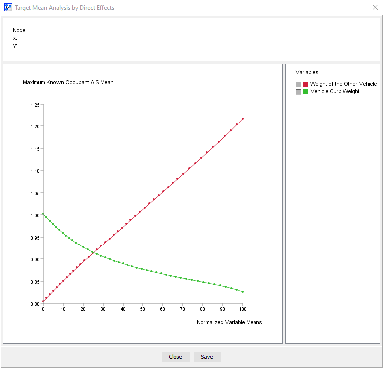
Our fleet-level model turns out to be adequate after all, and the Likelihood Matching algorithm does return results that appear similar to the results for the analysis of the Passenger Car model.

Simulating Interventions

Thus far, we have only computed the impact of reducing $\mathit{Vehicle\ Curb\ Weight}$ while leaving the distribution of Weight of the Other Vehicle the same. This means we are simulating as to what would happen if a new fleet of a lighter fleet of vehicles were introduced, facing the older, heavier fleet. This simplification may be reasonable as long as the new fleet is relatively small compared to the existing one. However, in the long run, the distribution of Weight of the Other Vehicle would inevitably have to become very similar to GV_CURBWGT.

In order to simulate such a long-run condition, any change in the distribution of $\mathit{Vehicle\ Curb\ Weight}$ would have to be identically applied to Weight of the Other Vehicle. This means once we set evidence on $\mathit{Vehicle\ Curb\ Weight}$ (and fixed its distribution) we need to set the same distribution on Weight of the Other Vehicle (and fix it).

Note that we are now performing causal inference, i.e. “given that we do” versus “given that we observe.” Instead of observing the injury risk of lighter vehicles (and all the attributes and characteristics that go along with such vehicles), we do make them lighter (or rather force them by mandate), while keeping all the attributes and characteristics of drivers and accidents the same.

For instance, reducing the average weight of all vehicles to 1,500 kg appears beneficial. The risk of serious or fatal injury drops to 2.85%. Considering these simulated results, this may appear as a highly desirable scenario. This would theoretically support a policy that “lightens” the overall vehicle fleet by government mandate. However, we must recognize that such a scenario may not be feasible as functional requirements of vans and trucks could probably not be met within mandatory weight restrictions.

Alternatively, we could speculate about a scenario in which there is a bimodal distribution of vehicle masses. Perhaps all new passenger cars would become lighter (again by government mandate), whereas light trucks would maintain their current weights due to functional requirements. Such a bimodal scenario could also emerge in the form of a “new and light” fleet versus an “old and heavy” existing fleet. We choose a rather extreme bimodal distribution to simulate such a scenario, consciously exaggerating to make our point.

As opposed to a homogeneous scenario of having predominantly light vehicles on the road, this bimodal distribution of vehicles increases the injury risk versus the baseline. This suggests that a universally lighter fleet, once established, would lower injury risk, while a weight-wise diverse fleet would increase risk.

These simulations of various interventions highlight the challenges that policymakers face. For instance, would it be acceptable, with the objective of long-term societal safety benefit, to mandate the purchase of lighter vehicles, if this potentially exposed individuals to increased injury risk in the short term? What are the ethical considerations with regard to trading off “probably more risk now for some” versus “perhaps less risk later for many”? It appears difficult to envision a regulatory scenario that will benefit society as a whole, without any adverse effects to some subpopulation, at least for some period of time. However, it clearly goes beyond the scope of our paper to elaborate on the ethical aspects of weighing such risks and benefits.