Bayesian Network Properties

It is necessary to emphasize that, despite the visual nature of a Bayesian network, it is not a visualization of data. Rather, it is the structure that is visualized. So, what we see is the model, not the data. The Bayesian network is meant to be a generalization of the underlying data, rather than a “bit-perfect” replica of the data. Theoretically, and at a huge computational cost, a fully-connected Bayesian network can produce a perfect fit. However, that would bring us back to nothing more than the raw data, instead of generating an interpretable abstraction of the data.

Omnidirectional Inference

Any network that we see here is a fully specified and estimated model that can be used for inference. A particularly important property is what we call “omnidirectional inference.” While traditional statistical models usually contain one dependent and many independent variables, that distinction is not necessary for a Bayesian network. In fact, all variables can be treated equivalently, which is particularly interesting for exploratory research.

To gain familiarity with all the interactions learned from the data, we will experiment with omnidirectional inference and run various exploratory queries on different subsets of the model.

Example 1: Number of Lanes, Deformation Location, and Speed Limit

In Validation Mode, double-clicking on an individual node, or on a selected set of nodes, brings up the corresponding Monitors on the righthand-side Monitor Panel. Conversely, double-clicking again would remove them.

Click to Zoom

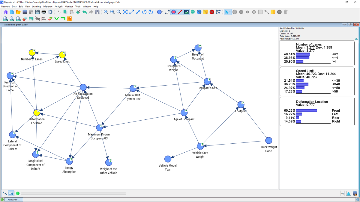
For instance, we show the Monitors for $\mathit{Number\ of\ Lanes}$, $\mathit{Speed\ Limit}$, and $\mathit{Deformation\ Location}$. Small histograms will show us the marginal distributions of those variables.

We can see that of all accidents 38.96% occur on roads with 3 or 4 lanes, or that 17.23% happen in areas with speed limits greater than 50 mph.

We might now want to ask the question, “what is the distribution of impact angles for accidents that happen on roads with more than 4 lanes?” We can use the network to answer this query by “setting evidence” via the Monitor for $\mathit{Number\ of\ Lanes}$. In BayesiaLab, this simply requires a double-click on the “>4” bar of this Monitor. Upon setting the evidence, the $\mathit{Number\ of\ Lanes}$>4 bar turns green, and we can now read the posterior probability distributions of the other nodes.

We see, for instance, that the share of left-side collisions $(\mathit{Deformation\ Location}=\mathit{Left})$ has dropped from 16.27% to 9.22%. However, we can observe another change. Given that we are focusing on roads with 5 or more lanes, now only 8.69% have a speed limit of 30 mph or below. In the marginal distribution, this share was 21.54%. The little gray arrows indicate the amount of change versus the previous distribution.

The Maximum Variation of Probabilities can be displayed by selecting Monitor > Highlight Maximum Probability Variations.

It is now obvious that one piece of evidence, i.e. setting $\mathit{Number\ of\ Lanes}$>4, has generated multiple updates to other variables’ distributions as if we had multiple dependent variables. In fact, all variables throughout the network were updated, but we only see the changes in distributions of those nodes that are currently shown in the Monitor Panel.

We now set the second piece of evidence, $\mathit{Speed\ Limit}$>50.

As a result, we see a big change in $\mathit{Deformation\ Location}=\mathrm{Rear}$, i.e. rear impacts; their probability jumps from 9.10% to 17.29%. Again, this should not be surprising as roads with more than 4 lanes and with speed limits of 50 mph or higher are typically highways with fewer intersections. Presumably, less cross-traffic would cause fewer side impacts.

Before we proceed, we remove all evidence and reset the Monitors to their marginal distribution. This can be done by right-clicking on the background of the Monitor Panel and selecting Remove All Observations from the Contextual Menu.

Once all evidence is removed, we can set new evidence. More specifically, we want to focus on side impacts on the driver’s side only, which can be expressed as $\mathit{Deformation\ Location}=\mathrm{Left}$.

Now the probability of $\mathit{Number\ of\ Lanes}$>4 has decreased and the probability of $\mathit{Speed\ Limit}$ $\le 30$ has increased. One can speculate that such kinds of collisions occur in areas with many intersections, which is more often the case on minor roads with fewer lanes and a lower speed limit.

This demonstrates how we can reason backward and forwards within a Bayesian network, using any desired combination of multiple dependent and independent variables. Actually, we do not even need to make that distinction. We can learn a single network and then have a choice regarding the nodes on which to set evidence and the nodes to evaluate.