From a Single Question to a Full Bayesian Network Model
How AI-Assisted Knowledge Elicitation Builds Supply Chain Intelligence in Six Steps
Dr. Lionel Jouffe
February 17, 2026
The EV battery supply chain is one of the most complex industrial ecosystems on the planet. It stretches from cobalt mines in the DRC and lithium brines in Chile to gigafactories in Germany and recycling plants in China. Geopolitical tensions, raw material scarcity, regulatory upheaval, technology disruption: the variables are overwhelming, and they are all interdependent.
How do you model something this complex? How do you go from a blank page to a quantified, probabilistic model that captures hundreds of causal relationships, assigns strengths, and lets decision-makers run what-if scenarios?
This article walks through a recommended workflow, from a single open-ended question to a fully operational Bayesian network, using AI-assisted knowledge elicitation. Each step produces a distinct type of graph, each more structured and more quantified than the last, forming a progressive exploration pipeline that turns unstructured domain knowledge into decision-ready intelligence.
A word of epistemological honesty before we begin. Each of these six representations is, by construction, a simplified projection of an overwhelmingly complex reality. Like shadows on the wall of Plato’s cave, or the forms glimpsed through the veil of Maya, none of them is the supply chain; they are partial, complementary views of it. As George Box famously put it, all models are wrong, but some are useful.
The value of this pipeline lies precisely in the diversity of perspectives it offers: semantic, relational, causal, probabilistic, risk-oriented. No single model captures the full picture, but together they illuminate far more than any one of them could alone.
The Starting Point: One Question
Everything begins with a single prompt fed to Hellixia, the AI assistant integrated into BayesiaLab and HellixMap:
Resilience and Profitability Analysis of the EV Battery Supply ChainFrom this open-ended question, the analyst initiates a structured exploration of the domain that will produce six progressively richer representations. No dataset is required at this stage. No expert panel. Each model is generated by the user through Hellixia, either in HellixMap for qualitative exploration and visualization, or in BayesiaLab for model editing and probabilistic inference.
The workflow described here is the one I recommend for apprehending a new domain and building understanding before constructing an operational decision model.
Step 1: Semantic Network - Mapping the Landscape
What It Is
The Semantic Network is a representation specific to the Bayesia ecosystem, built through a well-defined three-step workflow:
- Dimension Elicitation: the user selects domain keywords (here: Aspects, Characteristics, Components, Criteria, Dimensions, Elements, Factors, Features, Indicators, and Variables) that guide Hellixia in extracting the relevant dimensions of the domain. In this case, 93 dimensions were identified.
- Embedding Generation: for each dimension, an embedding is computed from its name and associated description.
- Structural Learning: BayesiaLab’s Maximum Weight Spanning Tree (MWST) algorithm selects the strongest pairwise semantic correlations to build a connected tree representing the overall structure of the domain’s vocabulary.
An optional but valuable enrichment step is Hellixia’s Verbalize Relationship function, which assigns a descriptive verb to each edge, making the network more readable.
It is essential to note that these relationships represent semantic proximity, not causation. Two concepts are linked because they are close in embedding space, not because one causes the other.

Analysis of the Network
The resulting network of 93 nodes and 92 edges reveals the semantic architecture of the EV battery supply chain domain. Five dimensions stand out by their connectivity:
- Manufacturing Capacity (8 connections) emerges as the most central concept, bridging production, resources, market demand, and financial performance.
- Supplier Diversification (6 connections) acts as a semantic bridge between supply chain visibility, temporal resilience, technical dimensions, vertical integration, and risk management.
- Supply Chain Visibility groups digital and traceability concerns.
- Temporal Resilience captures buffer stocks, disruption frequency, and recovery time.
- Technological Innovation captures cost competitiveness, breakthroughs, and modular design.
Together, these five dimensions organize the domain around three poles: industrial capacity, supply security, and innovation.
Step 2: Knowledge Graph - Structuring the Knowledge
What It Is
A Knowledge Graph (KG) is a directed, multi-relational graph where each arc carries an explicit verb (extracts, threatens, enhances) that qualifies the nature of the relationship between two concepts. Unlike the Semantic Network, the KG is not constrained to be a tree: nodes can have multiple parents and children, and cycles are permitted, enabling richer structural representations.
The relationships are directional and semantically typed, making the KG a more expressive tool for representing domain knowledge.

Analysis of the Graph
The Knowledge Graph condenses the domain into 40 nodes organized across 7 thematic classes (Supply Chain Stages, Risk Factors, Innovation, Strategic Management, etc.). Two nodes stand out as pure sinks:
- Profitability (15 incoming connections, zero outgoing)
- Resilience (9 incoming connections, zero outgoing)
Everything in this knowledge structure converges toward these nodes without feedback from them, confirming their status as the ultimate outcome variables of the domain.
Raw Material Extraction (10 connections, 5 in, 5 out) is the primary operational hub. Notably, the graph naturally captures the circular economy loop: End-of-Life Management → Raw Material Extraction, materializing the recycling feedback that is central to the industry’s future.
Step 3: Causal Semantic Diagram - Focusing on Causation
What It Is
The Causal Semantic Diagram (CSD) is a variant of the Knowledge Graph generated with a causal-only constraint. While the general KG admits any type of relationship (membership, attribute, functional, spatial, temporal), the CSD is produced from the outset with the restriction that every arc must express a causal mechanism (reduces, threatens, enables, stimulates).
The result is a graph directly interpretable as a map of the domain’s influence mechanisms, and a natural foundation for building a quantitative causal model.

Analysis of the Diagram
The CSD distills the domain to 20 nodes and 37 arcs with a remarkably convergent causal structure. Eight root causes feed into the network:
- Geopolitical Risks
- Environmental Sustainability
- Investment Capital
- Vertical Integration
- Strategic Partnerships
- Quality Control
- Logistics Efficiency
- Diversification Strategies
These converge toward a single terminal sink: Profitability (7 incoming arcs, zero outgoing).
Resilience (9 incoming arcs) is quasi-terminal, with a single outgoing arc (stabilizes Profitability), materializing the key causal link between the two KPIs. The node (6 inputs, 1 output) acts as a financial bottleneck where six distinct causal pathways converge on raw materials, technology, recycling, economies of scale, logistics, and regulation, before propagating to profitability.
Step 4: Causal Bayesian Network - Quantifying the Positive
What It Is
The Causal Bayesian Network (CBN) is a fully specified Bayesian network. Unlike the KG and CSD, every arc carries a quantified direct effect (positive or negative), enabling assessment not only of direction but also of the intensity and sign of each influence.
Generation is constrained by a node typology:
- Root Cause
- Intervention
- Confounder
- Intermediate Cause
- Effect
- Main Criterion
The quantification relies on direct effects combined via a Dual Noisy-OR model.

Analysis of the Network
The CBN comprises 50 nodes and 72 arcs. Its structure is strongly convergent: 22 Root Causes and 10 Interventions (28 parentless nodes total) feed, through 6 Confounders and 5 Intermediate Causes, into 6 Effects and one central Main Criterion, “High Resilience and Profitability of EV Battery Supply Chain,” which alone has 20 connections (14 in, 6 out).
The quantified direct effects reveal contrasting influences: some arcs carry strongly positive values (+85, +90), others sharply negative (−45, −60), immediately identifying favorable levers and risk factors. This quantification is the CBN’s primary added value over the qualitative representations.
Step 5: Risk-Centric Causal Network - Quantifying the Negative
What It Is
The Risk-Centric Causal Network (RCCN) adopts the complementary perspective to the CBN. Where the CBN models the conditions for achieving the main criterion, the RCCN focuses on its failure, i.e., the vulnerability of the system. Structurally, the RCCN is a probabilistic Bow-Tie: threats converge toward a central risk node, then diverge into consequences, with barriers on both sides.
Like the CBN, it uses a Dual Noisy-OR quantification and constrained node classes, but with a risk-specific typology:
- Threat (external risk driver)
- Preventive Barrier (upstream control)
- Sub-Risk (intermediate risk)
- Main Risk (central risk)
- Consequence (final impact)
- Mitigating Barrier (downstream control)
Each arc carries a quantified direct effect: positive for risk amplifiers, negative for protective factors.

Analysis of the Network
The RCCN comprises 87 nodes and 86 arcs. The bow-tie structure is clearly visible: 10 Threats feed 10 Sub-Risks, which converge toward the central Main Risk, “EV Battery Supply Chain Vulnerability” (19 connections: 10 in, 9 out), then diverge into 9 terminal Consequences (Revenue Loss, Profitability Erosion, Production Disruption, Financial Distress, etc.).
On either side, 30 Preventive Barriers act upstream on Sub-Risks (negative effects, e.g., −75, −70) while 27 Mitigating Barriers attenuate Consequences downstream. The highest threat effects reach +90 (Geopolitical Supply Concentration, Quality and Safety Incidents), and the strongest protections −75 (Capacity Planning, Quality Management Systems). The predominance of barriers (57 protective nodes out of 87) reflects a modeling approach oriented toward identifying risk control levers.
Step 6: Unconstrained Bayesian Network - Full Expressiveness
What It Is
The final type of network generated is an unconstrained causal Bayesian network. Unlike the CBN and RCCN, it imposes no predefined node classes (Root Cause, Threat, etc.) and no binary propositions. Nodes can have a variable number of symbolic states (here 3 to 5 states per node, e.g., Fragile / Moderate / Resilient / Highly_Resilient), or even be continuous variables, discretized variables, or Decision and Utility nodes in the case of an influence diagram.
Crucially, the quantification no longer relies on simple direct effects combined through a Dual Noisy-OR: the conditional probability tables (CPTs) are elicited directly, enabling the capture of non-linear interactions and more complex dependencies between variables. This is the most expressive representation in the generation chain.
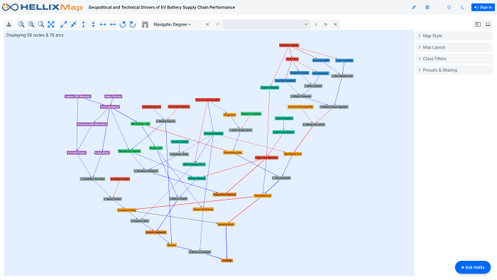
Analysis of the Network
The network comprises 56 nodes and 76 arcs, all chance nodes (no Decision or Utility nodes in this case). The topology is more distributed than the CBN or RCCN: 11 exogenous root nodes feed the network, which converges toward two terminal nodes: Profitability and Supply Chain Resilience.
The most connected nodes are Technology Maturity (6 connections), Recycling Capability (5), and Supply Chain Disruption (5), reflecting the pivotal role of technological readiness and circularity. Each node has at most 2 parents, keeping CPTs at a manageable size (≤ 9 cells) while enabling rich quantification. Arc thicknesses (from 1.0 to 2.80) convey the variable intensity of causal influences.
Bringing It All Together: From Generated Model to Decision Tool
The six graphs described above form the knowledge elicitation pipeline. The unconstrained Bayesian network (Step 6) is the one that serves as the foundation for the operational model. But unlike the five previous representations, which are generated directly by Hellixia, this final step requires significantly more human-AI interaction. The task is inherently more complex: fully specified conditional probability tables must be reviewed and validated, not merely generated.
In practice, this means working through Hellixia’s Conversational Network Modeler to verify the coherence of CPTs (inversions are frequent, especially for negative causal relationships), to add nodes where the model reveals gaps, and to reduce complexity by introducing latent variables using BayesiaLab’s divorcing technique. The result is no longer a one-shot generation; it is an iterative co-construction between the analyst’s domain expertise and the AI’s structural proposals.
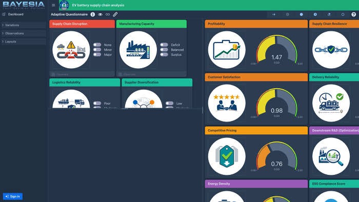
The operational network published as a WebSimulator is this refined version of the unconstrained BN: 56 nodes and 76 arcs, enriched with 16 pre-built scenarios based on real-world situations, including:
- China-Taiwan supply crisis
- DRC conflict
- Indonesia nickel ban
- EU Battery Regulation
- Solid-state breakthrough
- BYD cost pressure
It also includes a full WebSimulator interface definition that classifies nodes as Input, Output, or Hidden.
The WebSimulator is an interactive web-based interface where stakeholders can set input variables and observe how the network propagates their choices through the entire causal structure, all the way to profitability and resilience outcomes. No Bayesian network expertise is required to use it. Scenarios can be loaded with a single click to instantly explore what-if situations during client workshops.
Why This Matters
In the Bayesia ecosystem, there are three sources for constructing Bayesian networks: machine learning on data (structured or unstructured), brainstorming (expert-driven knowledge elicitation workshops), and Hellixia (AI-assisted generation). These three sources are not mutually exclusive; any combination can be used within a single project depending on data availability, expert access, and project constraints. What remains constant, however, is that expert validation is always required.
No model, however it was built, should be deployed without domain expert review.
The workflow described in this article illustrates the Hellixia pathway. Its primary value is in domain exploration and understanding: each step generates a different representation that illuminates a different facet of the problem space: semantic structure, knowledge relationships, causal mechanisms, quantified effects, risk architecture, and full probabilistic dependencies.
This progressive exploration provides a transparent, auditable path from question to comprehension, and ultimately to a model ready for decision support.
For the EV battery supply chain specifically, this approach surfaces insights that matter for OEMs, cell manufacturers, mining companies, investors, insurers, and policymakers alike: which factors truly drive resilience? Where are the financial bottlenecks? What are the highest-impact intervention points? What happens when geopolitics shifts?
The answer to all of these questions is not a single number. It is a structure, and building that structure, quickly and rigorously, is what this workflow delivers.
The Pipeline at a Glance
| Step | Graph Type | Nodes | Arcs | Nature | Key Feature |
|---|---|---|---|---|---|
| 1 | Semantic Network | 93 | 92 | Correlations | Undirected MWST from embeddings |
| 2 | Knowledge Graph | 40 | 72 | Typed relations | Multi-relational, cycles allowed |
| 3 | Causal Semantic Diagram | 20 | 37 | Causal verbs | Causal-only constraint, cycles allowed |
| 4 | Causal Bayesian Network | 50 | 72 | Quantified effects | Node typology + Dual Noisy-OR |
| 5 | RCCN | 87 | 86 | Risk quantification | Bow-Tie + Node typology + Dual Noisy-OR |
| 6 | Unconstrained BN | 56 | 76 | Full CPTs | Multi-state, direct elicitation |
| 6+ | Operational BN (WebSim) | 56 | 76 | Full CPTs | + Scenarios + WebSimulator |
A Note on This Example
I should be transparent: I am not a specialist of the EV battery supply chain. This article is purely an illustration of what is possible within the Bayesia ecosystem (BayesiaLab, Hellixia, HellixMap, and the WebSimulator), not a validated analysis of the domain.
For a real project, each of the generated models would need to be carefully reviewed with domain experts. The six graphs produced by the pipeline serve as a rich starting point, a structured canvas of dimensions, relationships, and causal mechanisms, from which experts can select, refine, and complement the variables to integrate into the final decision model.
They may add dimensions that the AI did not surface, remove those that are irrelevant, and, critically, validate every node’s states (for instance, defining precisely what the levels of Profitability or Revenue mean in practice) and every causal relationship. In this demonstration, I relied on common sense alone; a production model demands domain expertise at every step.
About the Author
Dr. Lionel Jouffe is co-founder and CEO of France-based Bayesia S.A.S. Lionel holds a Ph.D. in Computer Science from the University of Rennes and has worked in Artificial Intelligence since the early 1990s. While working as a Professor/Researcher at ESIEA, Lionel started exploring the potential of Bayesian networks. After co-founding Bayesia in 2001, he and his team have been working full-time on the development of BayesiaLab. Since then, BayesiaLab has emerged as the leading software package for knowledge discovery, data mining, and knowledge modeling using Bayesian networks. It enjoys broad acceptance in academic communities, business, and industry.