Tutorial: Optimizing Customer Loyalty
An Integrated Market Research Workflow Using Bayesian Networks and BayesiaLab
Executive Summary
Identifying Priorities for Maximizing Repurchase Intent
This tutorial illustrates an innovative market research workflow for deriving marketing and product planning priorities from auto buyer surveys. In this study, we utilize the Strategic Vision New Vehicle Experience Survey, which includes, among many other items, customers’ satisfaction ratings with regard to over 100 individual product attributes.
Challenge: Indistinguishable Drivers of Loyalty
With traditional statistical methods, it has been difficult to rank the importance of individual product attribute ratings with regard to an overall measure, such as repurchase loyalty.
The key challenge is that customers’ ratings of individual product attributes are highly correlated. When plotted, we see 100 lines that are nearly indistinguishable in terms of their slope. Given this collinearity of all variables, traditional statistical methods fail to distinguish the importance of individual ratings. We could only naively conclude that an improvement in any rating would generally be associated with higher loyalty. No clear priorities could be established on such a basis.
Solution: Bayesian Networks as Modeling Framework
To overcome this problem, we employ an alternative framework: we use Bayesian networks as the mathematical formalism, plus the machine-learning and optimization algorithms of the BayesiaLab software package. This approach embraces collinearity as a feature in the model, instead of suppressing it as a nuisance.
Implementation
First, using BayesiaLab, we machine-learn a Bayesian network that models customers’ brand loyalty as a function of their ratings of their current vehicle. This identifies key factors as loyalty drivers in the overall market, at the segment level, and finally at the model level. With these factors identified, we perform optimization for each vehicle within its competitive context. As a result, we obtain a list of specific priorities for each vehicle, along with the simulated gain in loyalty.
Other Benefits
No Black Box
Many modeling techniques offered in the field of marketing science are opaque to the end user of the research. The nature of many models makes them inherently black-box, and thus requires a leap of faith by the decision-maker.

Not so in our research framework with Bayesian networks. Regardless of one’s quantitative skills, any subject matter expert can, by simply using common sense, interpret the Bayesian network models generated with our workflow. Any stakeholder can immediately scrutinize such a model, thus enabling him to verify its structure, or, by using his domain knowledge, to invalidate it. Their inherent falsifiability makes Bayesian networks ideal scientific tools.
Real-Time Recommendations
In most organizations, waiting for research results and their interpretation is a matter of months. The time span between a consumer sentiment expressed in a survey and a company’s response can sometimes even exceed the lifecycle length of a product.
Our workflow creates a single, direct, and transparent link from data to recommendation. This directness provides unprecedented analysis speed. We reduce the lag between receipt of data and delivery of recommendations from months to days. As a result, near real-time policy recommendations are feasible for the first time.
Introduction
Background
Market Maturity and Homogeneity
The auto industry is an example of a mature market. It is fair to say that all automakers offer high-quality products these days in North America. The proverbial “lemons” are few and far between. Fierce competition has led to product offerings that are remarkably similar for their respective vehicle category, both in their specifications and their functional performance. With similar cost and budget constraints, and an overlapping supplier base for all manufacturers, the auto business is mostly about eking out minute advantages, as opposed to creating fundamental breakthroughs.
No doubt, the brand plays a major role in buying decisions. Hence, marketing, branding, and promotion efforts of automakers typically absorb a similar amount of resources as the actual R&D expenses for vehicle development. For the purpose of this paper, however, we will not venture into the challenging domain of return on marketing investment. This is a topic for another methodology tutorial in the future.
Given this overall quality and performance homogeneity, consumer perceptions, as we will see in this study, are also remarkably homogeneous across similar kinds of vehicles. For market researchers, it is thus very difficult to “tease out” material differences in customers’ perception of product attributes of competitive vehicles. It is even more challenging to establish which of these similarly-perceived vehicle characteristics do really matter when it comes to buying an automobile.
Loyalty
“It is cheaper to keep a customer than to find a new one” is an often-quoted marketing adage. Loyalty is a very relevant quantity, much more tangible than mere satisfaction. Given the maturity of the auto market and rather lengthy ownership cycles, repurchase loyalty is of special significance. Thus, in this study we go beyond satisfaction and instead link product ratings to stated repurchase intent.
We will focus exclusively on how customers’ product ratings affect loyalty, i.e., what really matters for brand loyalty. We will present a methodology that identifies the relevance of minute differences in consumer perception to prioritize among a broad range of opportunities to improve product ratings.
Workflow Overview
Latent Factor Induction
In this paper, we employ BayesiaLab’s machine learning algorithms to generate Bayesian networks that will allow us to identify major concepts, i.e., latent factors, from the observed satisfaction ratings, i.e., manifest variables. Inducing factors creates a level of abstraction that will allow us to see a “bigger picture,” that is more stable than if it is only based on manifest variables. Once factors are identified, we will examine how they “drive” brand loyalty. Ultimately, we want to establish the effect of these factors with regard to the outcome variable, i.e., loyalty.
Multi-Level Analysis
We will examine loyalty drivers at multiple levels of the market. We will identify areas of opportunity for improving loyalty at both the segment level and the vehicle model level.
- Segment refers to a vehicle category, such as Subcompacts or Large Sedans. There are numerous segmentation schemes in the auto industry, each with its own terminology. However, automakers generally agree on the definition of the Full-Size Pickup segment, which is the focus of this study.
- Vehicle model refers to a make (brand) and model/line, e.g., Ford Explorer or Nissan Altima. In this case study, we do not drill down to the trim level, e.g., Ford Explorer Limited or Nissan Altima 2.5 S.
More specifically, we will proceed from the overall market to the Full-Size Pickup segment, and then to the vehicle models within it. We chose this particular segment primarily for expository simplicity. It is a very well-defined segment in terms of vehicle characteristics while consisting of only a few major contenders. Plus, it is one of the most important segments in the U.S. auto industry, both in terms of volume and profitability.
Optimization
Once loyalty drivers are modeled, we will identify priorities for improvements by vehicle model. For each model, in its specific competitive context, our approach will generate recommendations with the objective of improving brand loyalty.
As we examine the impact of satisfaction ratings on loyalty, we need to remember, though, that satisfaction ratings are inherently subjective. The recommendations we will present do not necessarily specify the means by which ratings should be improved.
Acknowledgements
We would like to express our gratitude to Alexander Edwards, President of Strategic Vision, Inc. [3], for generously providing data from their 2009 New Vehicle Experience Survey for our case study.
Notation
To clearly distinguish between natural language, software-specific functions, and example-specific variable names, the following notation is used:
- Exact BayesiaLab commands, menu paths, and GUI labels are shown in backticks.
- Menu paths use the
>separator. - Example-specific names retain their exact capitalization when referenced directly.
[3] Strategic Vision is a research-based consultancy with more than 35 years of experience in understanding consumers’ and constituents’ decision-making systems for a variety of Fortune 100 clients, 10 Downing Street, Coca-Cola, American Airlines, Procter & Gamble, the White House, and most automotive manufacturers and many advertising agencies. The company specializes in identifying consumers’ complete motivational hierarchies, including product attributes, personal benefits, values/emotions, and images that drive perceptions and behaviors. Strategic Vision has at its core a large-scale syndicated automotive experience and “Pulse of the Customer” (POC) study that collects more than 350,000 responses annually, using over 1,500 comprehensive data points. Since its foundation in 1972 and incorporation in 1989, Strategic Vision, led by company founders Darrel Edwards, Ph.D., J. Susan Johnson, Sharon Shedroff, and Alexander Edwards, has used in-depth Discovery Interviews and Value Centered Survey instruments that provide comprehensive, integrated, and actionable outcomes, linking behavior to attributes, consequences, values, emotions, and images (www.strategicvision.com ).
Tutorial
Source Data
Our case study uses real-world data from the auto industry, which has conducted customer satisfaction research for decades. More specifically, we utilize the 2009 New Vehicle Experience Survey (NVES), a syndicated study conducted by Strategic Vision, Inc., which surveys new vehicle buyers in the U.S. This study is widely used in the auto industry, and it is one of the principal resources for market researchers and product planners. NVES contains over 1,000 variables and close to 200,000 respondent records. Among many demographic and psychographic variables, NVES contains 98 individual satisfaction measures, ranging from Acceleration to Wiper System Controls.
Data Selection
From the original NVES dataset consisting of 1,089 columns and 71,200 rows, we select 103 columns that are relevant for the purposes of this tutorial [4].
The first group of columns refers to the vehicle type, e.g., make, model, and vehicle segment. The second group includes 98 columns that all concern the vehicle buyer’s satisfaction with specific aspects of the purchased vehicle, ranging from Ability to Control Sound to Wiper System Controls.
For notational convenience, we rename a number of frequently used variables as follows:
- New Model Segment ➔ Segment
- New Model Purchased - Brand ➔ Make
- New Model Purchased (Alpha Order) ➔ Make/Model
- Rate Buy Another From Same Manufac. ➔ Loyalty
Coding
NVES measures all satisfaction-related variables on an ordinal scale, from 1 (A failure) to 5 (Delightful), as shown in the excerpt from the printed questionnaire.
[4] See the appendix for a complete list of the selected variables.
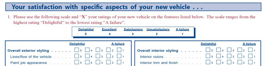
For analysis purposes, most market researchers have typically been using the NVES satisfaction ratings linearly transformed into a 1.5-9.5 scale. We will follow this convention in our tutorial.
Loyalty is asked in the NVES with the following question, which also features an ordinal scale for the response, ranging from Definitely will not to Definitely will.
Given that our objective is loyalty optimization, we need to associate a numerical value with each of the ordinal states of this response variable. The following linear assignment of probabilities is somewhat arbitrary, but for the purpose of this study we will accept it as a reasonable approximation.
| Response | Probability |
|---|---|
| Definitely Will Not | 0.00 |
| Probably Will Not | 0.25 |
| Do Not Know | 0.50 |
| Probably Will | 0.75 |
| Definitely Will | 1.00 |
Data Import
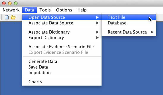
To start the analysis with BayesiaLab, we first import the survey dataset, which was provided as a CSV file [5]. With Data > Open Data Source > Text File, we start the Data Import Wizard, which immediately provides a preview of the data file.
[5] CSV stands for “comma-separated values,” a common format for text-based data files.
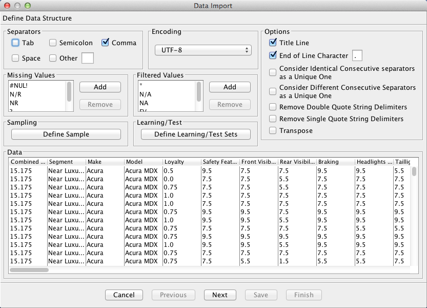
The table displayed in the Data Import wizard shows the individual variables as columns and the responses as rows. There are a number of options available, e.g., for sampling. However, this is not necessary in our example given the relatively small size of the database.
Clicking the Next button prompts a data type analysis, which provides BayesiaLab’s best guess regarding the data type of each variable.
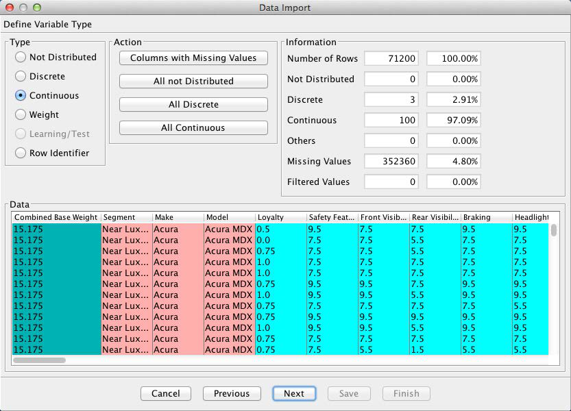
Furthermore, the Information box provides a brief summary regarding the number of records, the number of missing values [6], filtered states, etc.
In this example, we will need to override the default data type for the Combined Base Rate variable. This variable serves as the survey weight of each observation. We change the data type by highlighting the column and clicking the Weight check box, which changes the color of the Combined Base Rate column to green.
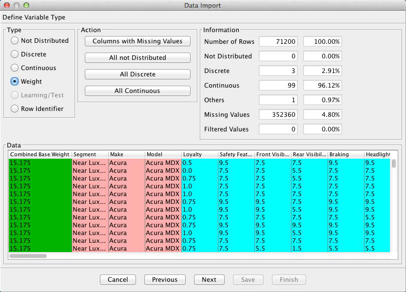
[6] There are no missing values in our database and filtered states are not applicable in this survey.
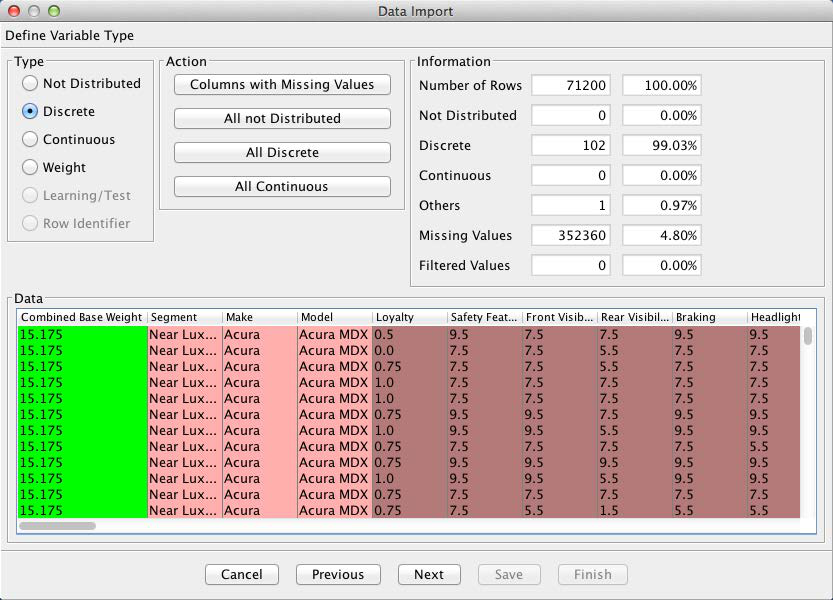
BayesiaLab interprets all the numerical columns as Continuous, which is technically correct. Consequently, BayesiaLab would attempt to discretize these variables. However, in our case, these variables were already discretized by the response levels given in the questionnaire. Thus, we will use this discretization as is. We do so by highlighting all continuous variables and then ticking the Discrete checkbox.
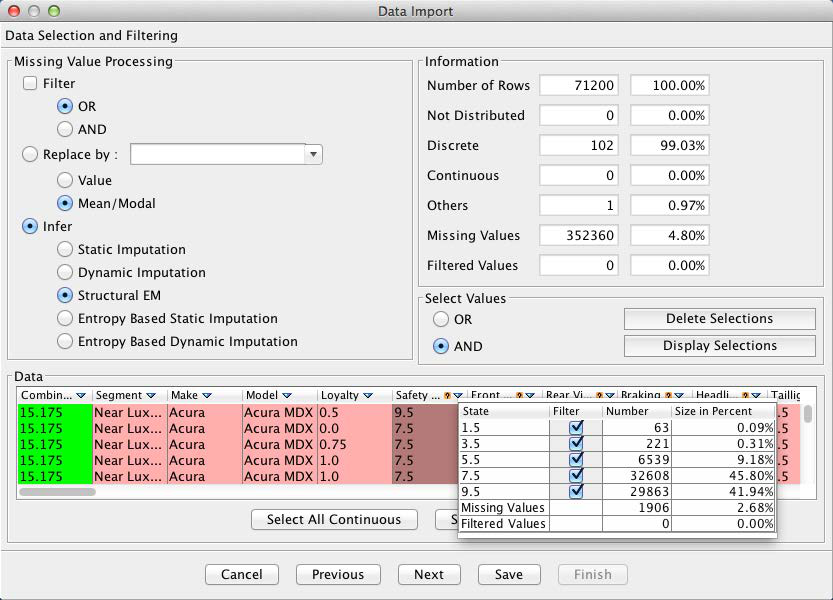
The next screen provides options as to how to treat any missing values. As shown by the Information panel, 4.8% of all values are missing in this dataset. Clicking the small upside-down triangle next to the variable names brings up a window with key statistics of the selected variable, in this case Loyalty.
Furthermore, columns with missing values are highlighted with a small question mark symbol. By highlighting any such variable, we are given the option of selecting the missing values imputation algorithm under the Infer section of the window.
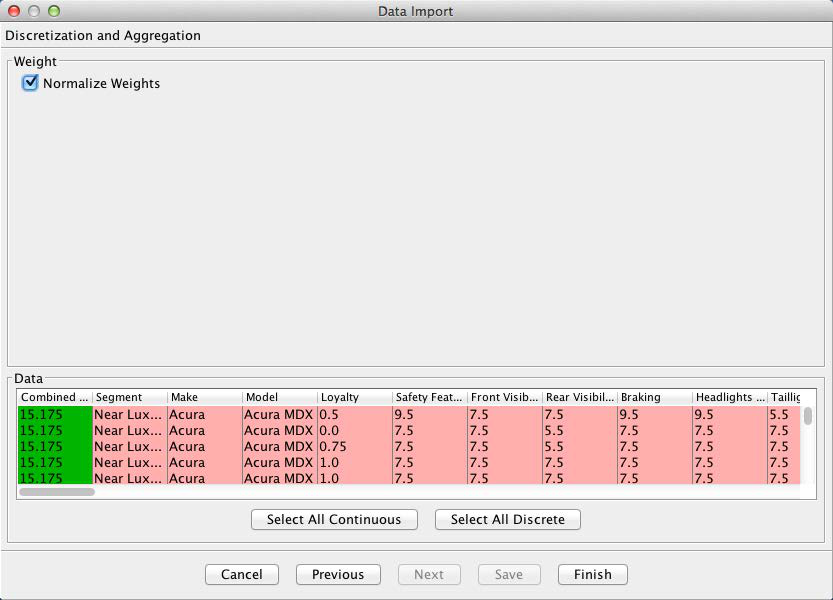
Given that we are using weights in this dataset, we now have an option to Normalize Weights. If we left this option unchecked, each record in the dataset would be counted as many times as the weight indicates. For instance, the first row would be counted 15.175 times. Applied to all rows, this would yield the correct proportion of observations relative to each other. However, BayesiaLab would subsequently end up “overlearning” from 3,233,840.85 weighted observations [7]. To avoid generating a false sense of precision, we select Normalize Weights, so each response, on average, represents one transaction.
[7] Each response in this survey, on average, represents roughly 45 vehicle purchases.
Upon completion of the import process, we obtain an initially unconnected network, which is shown below in the screenshot. All variables are now represented as nodes, one of the core building blocks in a Bayesian network. A node can stand for any variable of interest. Once the variables appear in this form in a graph, we will exclusively refer to them as nodes.
The wide spectrum of nodes can now be seen at a glance. For clarity, this network is shown without its graph panel window. Whenever the context is clear, we will present the network by itself in this tutorial.
Unsupervised Structural Learning
A central element in our study is to look for overarching concepts among the 98 satisfaction measures in our dataset. Once identified, these concepts will subsequently serve as factors as we further develop our model.
Machine learning a Bayesian network is a remarkably practical way to identify easily-interpretable variable clusters for factor induction. Among BayesiaLab’s Unsupervised Learning algorithms, the Maximum Weight Spanning Tree is a very efficient approach for quickly obtaining a Bayesian network that can provide the basis for variable clustering. The speed of this particular method is due to a key constraint, namely that in the network to be learned, each node is restricted to having only one parent node. This massively reduces the number of candidate networks that the learning algorithm must examine.
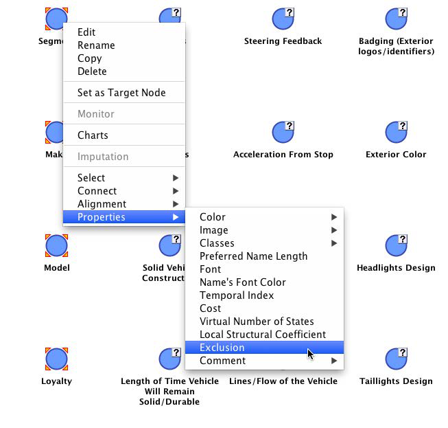
Prior to initiating clustering, we exclude any nodes that should not be part of the clustering process, such as the node we later use as the target node and nodes we use as breakout variables (e.g., Segment). We can exclude nodes by right-clicking selected nodes and choosing Properties > Exclusion from the contextual menu. Alternatively, hold X while double-clicking nodes. Once excluded, nodes appear in the excluded style shown below.
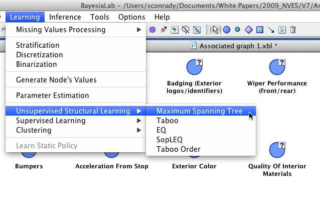
Now we can start the learning process from the main menu: Learning > Unsupervised Structural Learning > Maximum Spanning Tree.
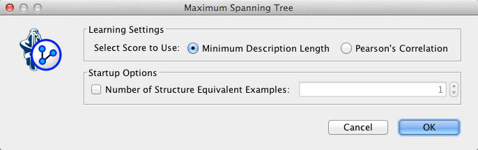
The Maximum Weight Spanning Tree is the only learning algorithm in BayesiaLab that offers an alternative to the Minimum Description Length (MDL) as the learning score. However, without further explanation, we will stick to the default and confirm MDL.
This default view of the resulting network is hardly intuitive. Hence, throughout this exercise, we will make frequent use of one of several available layout algorithms.
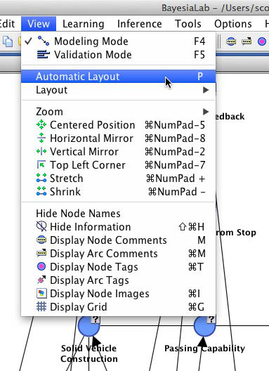
All layout algorithms are accessible from the main menu via View > Layout. Most often, we will use View > Automatic Layout, or alternatively use the shortcut P.

Upon applying a layout algorithm, we obtain an untangled version of the original network. Note that the structure of the network remains unchanged. We can further adjust the positions of the nodes as needed to create a legible and interpretable layout.
In this network, we can examine the probabilistic relationships between the nodes, which are represented as arcs. The structure of the network lends itself to a “sanity check” against our own domain knowledge. For instance, we can look at the lower right branch of the network and see that all these nodes relate to the vehicle interior and seating. It should not surprise us to see that Front Seat Roominess is directly connected to Ease of Front Seat Entry.
Mapping
Beyond this kind of qualitative assessment, BayesiaLab’s Mapping function is very helpful for interpreting the importance of the nodes and the strength of the relationships between them.
We can initiate Mapping from within the Validation Mode by selecting Analysis > Visual > Mapping.
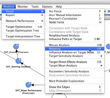
The Mapping window features drop-down menus for Node Analysis and Arc Analysis. We select Node Force for Node Analysis; for Arc Analysis, we choose Mutual Information.
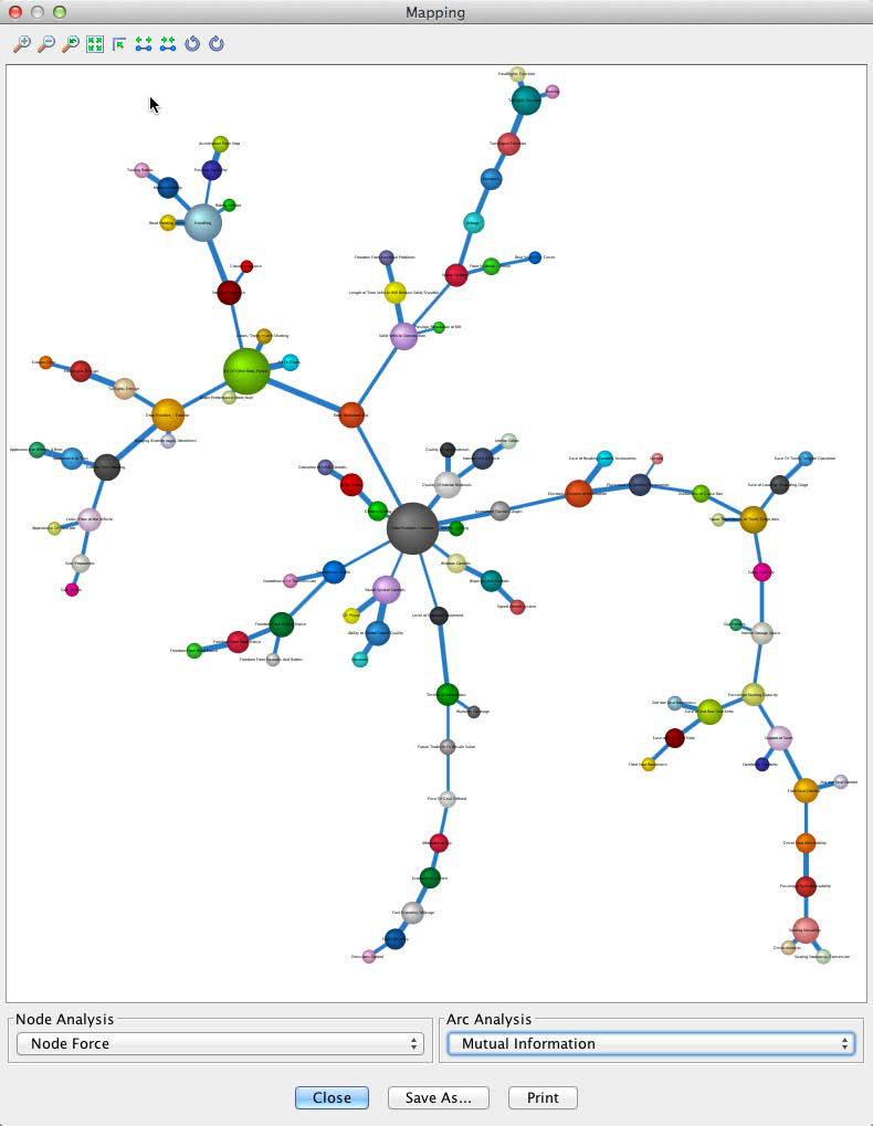
In the resulting graph, as selected, node size reflects the Node Force and arc thickness reflects the Mutual Information. This visualization suggests that Solid Vehicle Construction and Handling are among the most important nodes. All measures appear plausible, so we feel comfortable moving forward on this basis.
Missing Values Imputation
As we already saw during the data import process, all rating variables contain missing values. Given that we set Structural EM as the missing values imputation algorithm, we could proceed with our entire analysis without further thinking about the missing values. The Structural EM algorithm would handle them automatically as we go along [8]. However, there is a significant computational burden associated with this ongoing computation.
To accelerate all subsequent tasks, we will fix the most recent imputation that was generated during the learning of the Maximum Weight Spanning Tree.
To perform this imputation, we first select all nodes, then right-click on any one of the nodes with missing values, and finally select Imputation from the contextual menu.
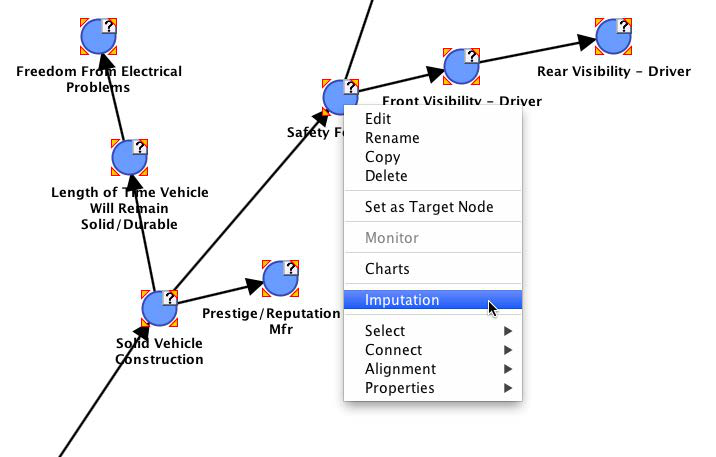
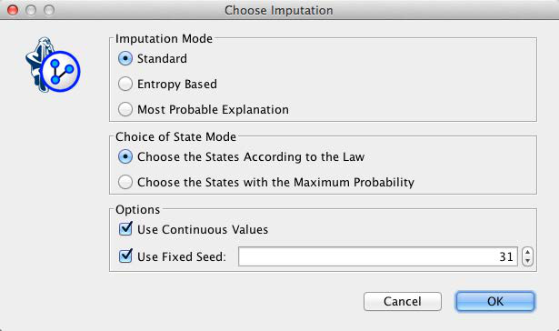
We are given a choice of modes, of which we select Standard and Choose the States According to the Law.
Upon completion of the process, all question marks disappear from the network, indicating that there are no more missing values.
[8] For more details, please see our white paper on missing values processing with Bayesian networks: http://bayesia.us/missing-values-processing-with-bayesian-networks.html
Variable Clustering
The network, as we see it here, is intended only as an interim step. For product planning or decision-making purposes, it would indeed be difficult to work directly with 98 manifest nodes. We would not be able to see the proverbial forest for all the trees. Rather, this network will serve as the basis for Variable Clustering, i.e., grouping nodes into meaningful concepts.
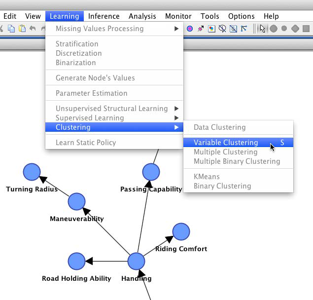
We start this clustering process, from within the Validation Mode, by selecting Learning > Clustering > Variable Clustering (or by using the keyboard shortcut S).
We now see the same graph as before; however, the nodes are now colored according to their proposed cluster membership. In our case, BayesiaLab suggests 26 clusters, as indicated in the menu bar.
We can move the slider to change the number of clusters (or by clicking the arrow buttons). This allows us to align the number of clusters with our domain knowledge. As we change the number, the node colors are automatically updated.
Additionally, we can view a dendrogram while adjusting the number of clusters. Two dendrogram examples are shown below: one with 27 clusters (left) and one with 10 clusters (right).
Alternatively, we can show the currently selected clustering in a format similar to the Mapping function via the menu bar.
For an easier interpretation of these “bubbles”, we can attach labels to them. Since each bubble represents a cluster of nodes, we select Display Best Node Name from the contextual menu.
This shows the name of the node that most strongly contributes to each cluster, given the currently selected number of clusters.
Two screenshots are shown as examples, based on 24 and 10 clusters respectively.
With Dendrogram and Mapping, we can visually experiment until the appropriate cluster number is established. The final selection of the number of clusters remains the task of the analyst. There is no hard-and-fast rule for choosing the number of clusters as this example illustrates. For instance, is it appropriate to cluster nodes related to noise with nodes related to smoothness? Two alternative Dendrograms are shown below. Only a domain expert can make a judgment in this regard.
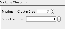
The number of clusters automatically proposed by BayesiaLab is based on two heuristics: the first is based on the strength of the relationships, the second on the maximum number of variables per cluster. Whereas we generally do not advise changing the former, the latter can be modified via Options > Settings > Learning > Variable Clustering.
After further review of all diagrams, we conclude that 24 clusters are most appropriate for this domain and confirm this choice by clicking the Validate Clustering button.
Furthermore, we confirm that we want to keep the colors from the just-completed interactive clustering.

This confirmation generates the Variable Clustering Report, which summarizes each node’s cluster membership.
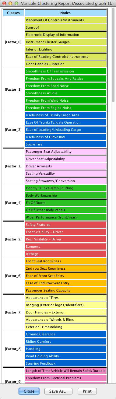
Initially, the clusters are simply labeled as [Factor_0], [Factor_1], …, [Factor_23] [9].
Latent Factor Induction via Multiple Clustering
As our next step, we introduce these newly-identified latent factors into our existing network and estimate their probabilistic relationships with the manifest variables. This means we create a new node for each latent factor, adding 24 new dimensions in our network. For this step, we need to return to the Modeling Mode because introducing factor nodes into the network requires learning algorithms.
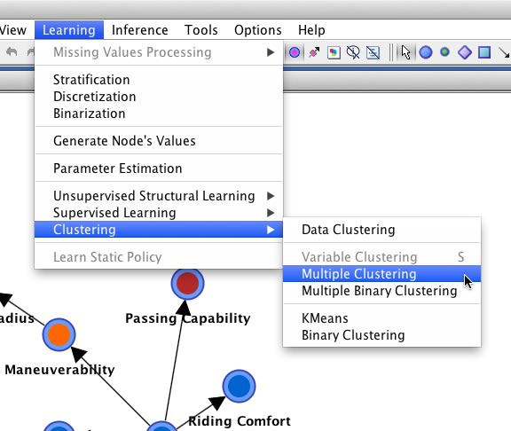
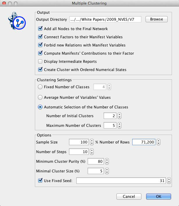
More specifically, we select Learning > Clustering > Multiple Clustering, which brings up the Multiple Clustering dialog.
There is a range of settings, but we will focus only on a subset of the available options. First, we need to specify an output directory for the learned subnetworks. Second, we need to set parameters for the clustering process, such as the minimum and maximum number of states that can be created during learning. For our example, we select Automatic Selection of the Number of Classes, which allows the learning algorithm to find the optimum number of factor states up to a maximum of five states. This means that each new factor will need to represent the corresponding manifest variables with up to five states [9].
[9] A complete list of factors and their associated nodes is provided in the appendix.
Upon completion of the Multiple Clustering process, we obtain a new network file that contains one small network for each cluster, with one factor being at the center of each cluster.
The arcs between the factors and their manifest nodes are labeled with Direct Effect Contribution values. This allows us to easily identify the importance of the manifests with regard to their respective factors.
Traditionally, we would now choose a name for each factor so we can interpret factors without looking at their manifests. For instance, , shown below, could be called Interior Quality or something similar. In BayesiaLab, we can defer this naming process by using the strongest node (based on Direct Effect Contribution) within each cluster as that factor’s Node Comment.
Clicking Display Node Comments in the menu bar will reveal Interior_Trim & Finish_(4) as a label on the factor. The suffix (4) indicates that 4 manifest variables are linked to this factor.


Factor States/Values
Beyond adding the factors to the network, the Multiple Clustering process has also generated states for all factors and computed their values. Inducing a factor means finding an appropriate summary of the underlying joint probability distribution defined by the manifest nodes. In the previous example of Factor_12, this would mean that the states of Factor_12 can summarize the following four nodes: Interior Trim & Finish, Quality of Interior Materials, Interior Colors, and Quality of Seat Materials.
We can examine the factor states and values by opening the network for Factor_12, switching into Validation Mode, and selecting all nodes for display in the Monitor Panel. By default, we see the marginal distributions of all the manifests and the factor.

By sequentially setting evidence on each of the four states of Factor_12, we see what states of the manifests correspond to the factor states.

Looking at these Monitors also provides some intuition regarding the values of the states of Factor_12. BayesiaLab computes these values as the weighted average of the associated manifests’ values. As such, Factor_12 becomes a compact summary of the connected manifest nodes.
Introducing the Target Node
Now that factors have been formally introduced into the network, each representing a major concept, we can proceed to the next step. We will introduce the principal variable of interest in this study, Loyalty, as the target variable.
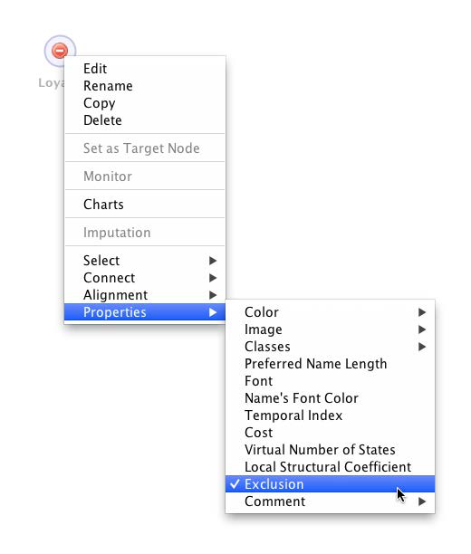
This node was excluded earlier in the clustering process, so it would not become clustered into a factor. So, the next step is to un-exclude this node, which we do by right-clicking the node and then selecting Properties > Exclusion (shortcut: press X and double-click on the node).
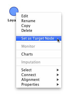
Also, we need to make this node the Target Node. We do this by picking Set as Target Node from the contextual menu. Note that the un-exclusion and the Target Node definition can be done at the same time by pressing T and double-clicking on the excluded node.
Upon introduction of the Target Node, we can interpret the status quo as the first two layers of a hierarchical model, as illustrated below. The outer ring contains the manifest nodes, the inner ring consists of the factors. In the middle, we have the yet-to-be-connected Target Node.
Focusing on Factors
We could continue our analysis with this network as is, including both factors and manifest nodes. However, for practical planning purposes, working with factors, i.e., the major concepts, is typically more relevant. Also, removing the manifest variables will improve the expository clarity of this tutorial. Thus, we will conduct all subsequent analyses exclusively with the factors, rather than the manifest nodes.
To delete the manifest nodes, we right-click on any one of them and then choose Select > Classes.
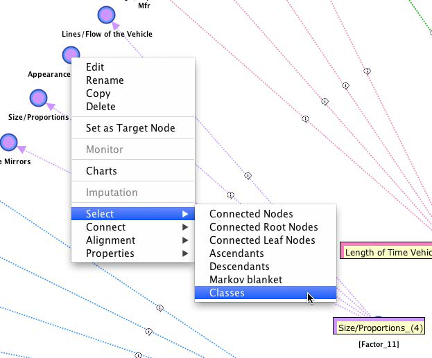
From the pop-up window, we pick Manifest.
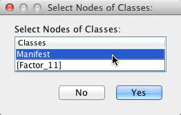
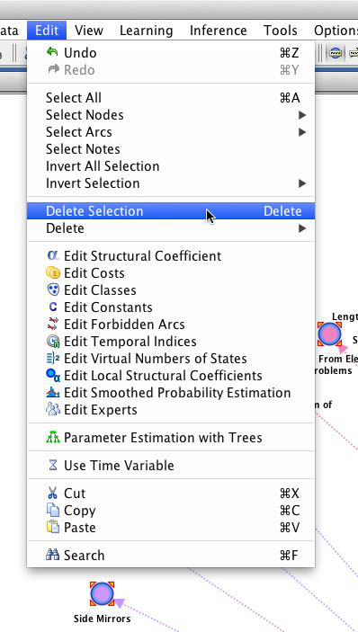
This highlights all manifest nodes, i.e., the outer ring. We can now delete them, either via the Delete key or from the main menu via Edit > Delete Selection.
This leaves us with the factors, the Target Node Loyalty, plus the previously excluded nodes, Segment, Make, and Model.
Supervised Learning
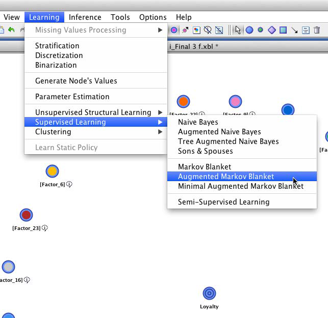
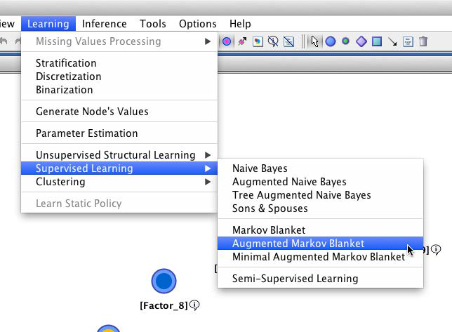
We can now use Supervised Learning to discover the relationships between the Target Node and the factors. We use the Augmented Markov Blanket, which is one of BayesiaLab’s Supervised Learning algorithms.
Using the default setting for the Structural Coefficient (SC=1), this learning algorithm yields the following network:
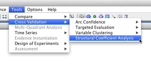
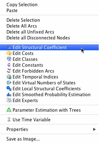
Structural Coefficient Analysis
In the newly-learned network, we see a total of 88 arcs connecting the 24 factor nodes and the target. Some nodes have up to five parent nodes, which implies a six-dimensional conditional probability table for those nodes. Given this relatively high level of network complexity, it is prudent to perform a Structural Coefficient Analysis: Tools > Cross Validation > Structural Coefficient Analysis.

This way we can examine, among other metrics, the data-to-structure ratio as a function of the structural network complexity.
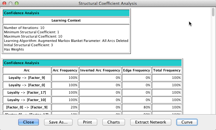
Once the report is presented, clicking Curve produces a kind of “scree plot”, which helps us identify a reasonable value of the Structural Coefficient. Unlike the scree plot we know from Factor Analysis, we read this plot from right to left.
By visual inspection of this graph, moving from right to left along the x-axis, we see an inflection point of the curve around SC=3. Below that value, the structural complexity is increasing faster than the data likelihood. Thus, we choose SC=3 and relearn the network on that basis with the Augmented Markov Blanket algorithm.
The resulting network is considerably simpler than before, now featuring only 65 arcs. Also, the Turning Radius and Taillights Function factors are no longer part of the network, which suggests that these two factors are least relevant with regard to loyalty.
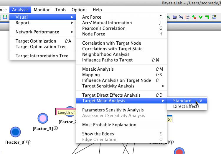
Target Mean Analysis
On the basis of this network structure, we can now examine the relationships between the factors and the target node. For this step, we select Analysis > Visual > Target Mean Analysis > Standard. This function computes the mean value of the Target Node by varying each factor, one at a time, across its entire range of values.
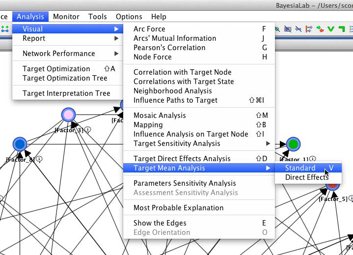
The Target Mean Analysis provides a quick overview of how our factor values are associated with the Target Node. The y-axis shows the mean values of the Target Node as a function of the factor values on the x-axis.
This plot suggests that all the factors are approximately linearly associated with the Target Node. Furthermore, the curves appear to run almost parallel between the x-values of 7.5 and 9. As a result, it is reasonable to formally compute “parameter estimates” for the slopes of these curves.
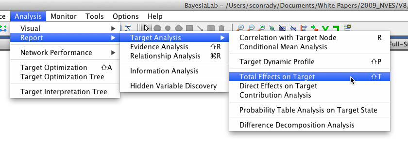
In BayesiaLab, this can be done by means of simulation via Analysis > Report > Target Analysis > Total Effects on Target. More specifically, BayesiaLab computes the derivative around the mean value of the x-range of each factor.
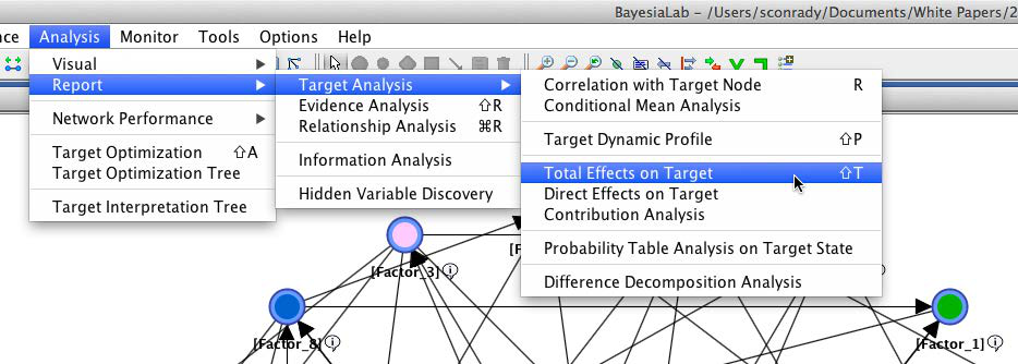
The results are presented in a table. The Total Effects column shows the change of the mean value of the Target Node, given the observation of a one-unit change in each of the factors. This value is what we commonly interpret as slope.
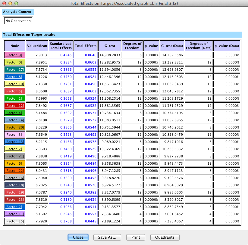
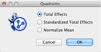
Clicking Quadrants on the report window shows a scatterplot with factor values on the x-axis and Total Effects on the y-axis. This allows us to better distinguish the factors, even though they have Total Effects in a fairly narrow range around 0.4 to 0.6.
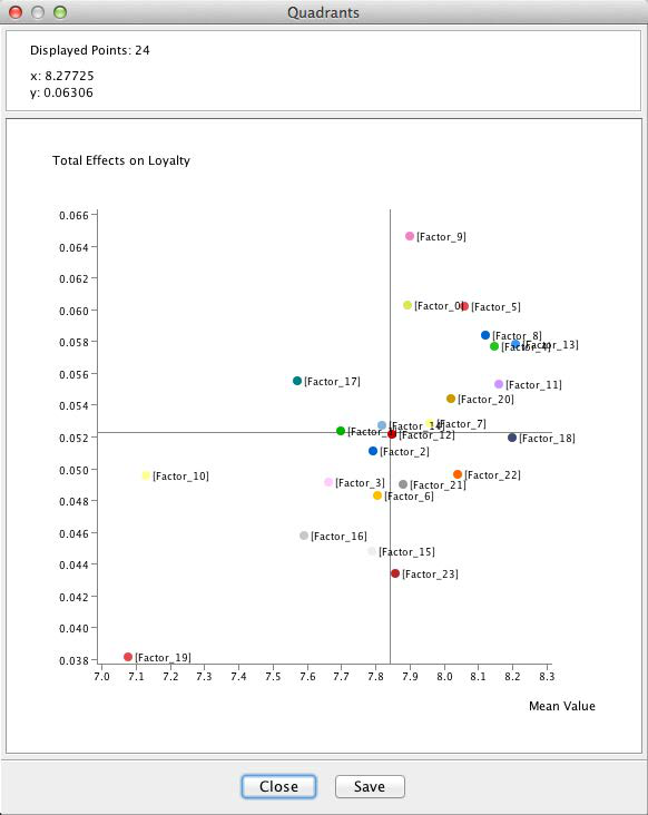
With the highest Total Effect, Length of Time Vehicle Will Remain Solid/Durable marks the top value on the y-axis of the plot. The factor Fuel Efficiency marks the bottom end on both axes. The position of the Fuel Efficiency factor is perhaps curious as our survey data covers 2009, when the auto industry was most severely affected by the recession.
However, as interesting as this may seem, it is probably of little practical use for planning purposes as this plot represents a view of the entire market, across all makes and all segments. It is reasonable to assume that effect heterogeneity exists between vehicle segments as different as Full-Size Pickups and Luxury Sedans.
Multi-Quadrant Analysis (Total Market ➔ Segment)
To study this domain at the level of vehicle segments, we could now start all over again and generate a new network for each segment from scratch. BayesiaLab provides a convenient shortcut for the researcher by means of Multi-Quadrant Analysis.

BayesiaLab can automatically replicate the original model (learned for the entire market) for each state of a specified Breakout Node. This is where the previously excluded node, Segment, comes into play. To make use of it here, we need to un-exclude it at this time.
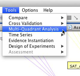
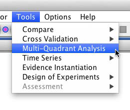
We start the Multi-Quadrant Analysis from the main menu, within Validation Mode, via Tools > Multi-Quadrant Analysis.
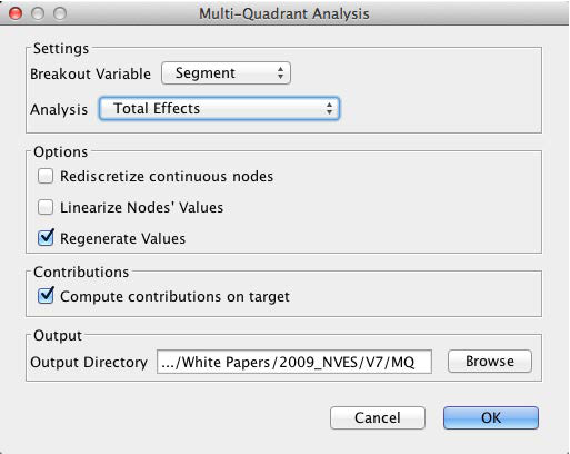
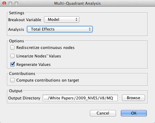
In the following dialog box, we specify the options of the Multi-Quadrant Analysis. Most importantly, we need to select the Breakout Variable, which in our case needs to be Segment. Furthermore, we define an output directory. This is where the segment-level networks will be saved.
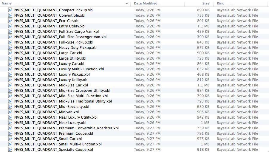
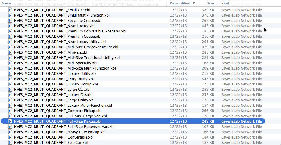
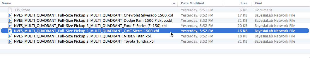
Once this process is completed, all new networks can be found in the specified directory. The file names are created according to the following syntax: Original Network File Name + MULTI_QUADRANT + Breakout Variable State.
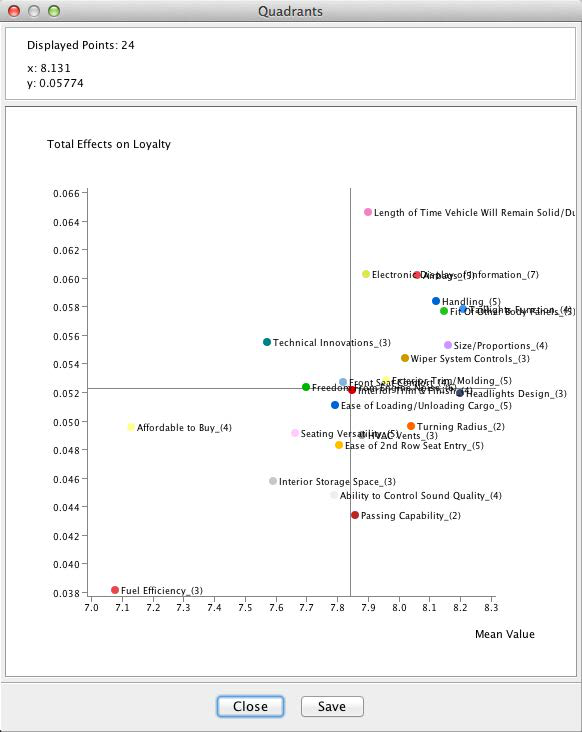
In BayesiaLab itself, we obtain a Quadrant Plot, which shows the Mean Value of each node on the x-axis and the Total Effect on the y-axis (even though quadrants are not explicitly shown here, we will soon explain how a quadrant view can be helpful for interpretation).
This plot exists for all the states of the Breakout Variable, i.e., for all segments. The currently selected state is highlighted.
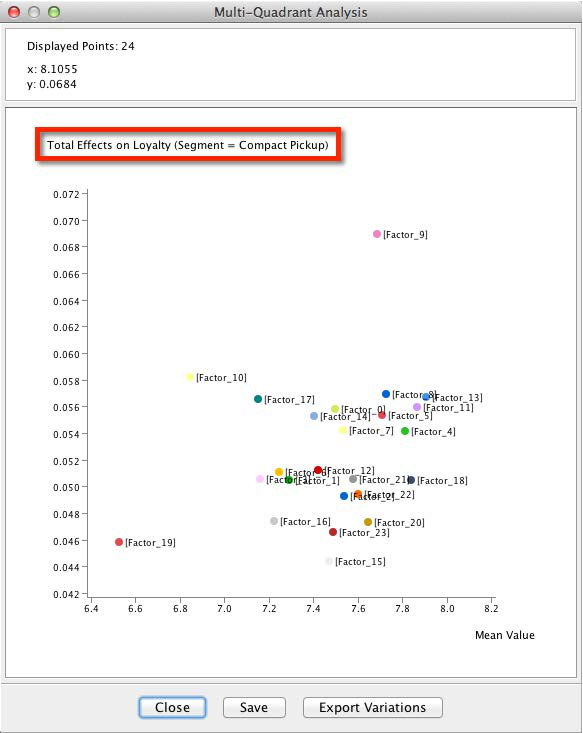
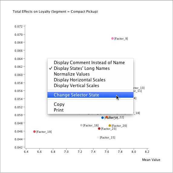
By default, the Breakout Variable’s first state is shown, in our case, Compact Pickup. To see the results of other segments, we right-click on the plot and pick Change Selector State.
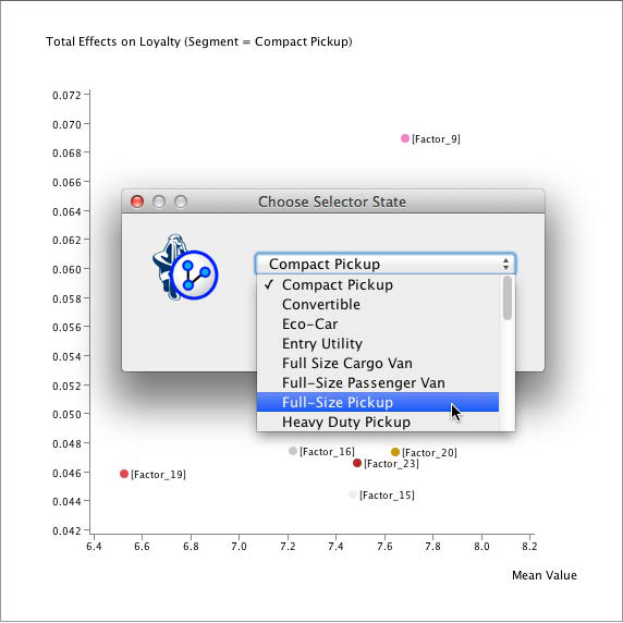
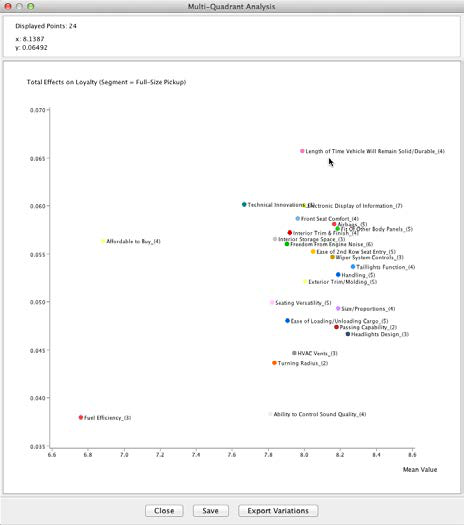
Full-Size Pickup Segment
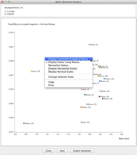
For reasons explained in the introduction, we will now focus on the Full-Size Pickup segment.
This plot allows immediate interpretation. The x-axis represents the mean satisfaction of Full-Size Pickup buyers with regard to the factors. The y-axis shows the Total Effect of each factor with regard to Loyalty. More specifically, the y-axis shows the value associated with a one-unit change in the respective factor. Casually speaking, we interpret this as the “importance” of a variable. For Full-Size Pickup, this means that Ability to Control Sound Quality is fairly unimportant for Loyalty. On the other hand, even though Affordable to Buy rates low on the x-axis, it rates fairly high on the y-axis, meaning it is rather important for Loyalty.
The following conceptual diagram shows a commonly used interpretation framework.
We should emphasize that we are interpreting factors, rather than manifest variables. Thus, the apparent “top driver” in the Full-Size Pickup plot, Length of Time Vehicle Will Remain Solid/Durable, is actually Factor_9. For convenience, we apply the name of the node that contributes most strongly to this factor as its node comment. For reference, the manifest nodes associated with this factor are shown below.
In the Quadrant Plot, we can easily toggle between the factor name, i.e., [Factor_x], and the Node Comment via the contextual menu.
All the factors’ positions on the Quadrant Plot become even more meaningful in the context of other segments. Within the same Quadrant Plot window, we can hover over any of the factors to see how other segments compare on the selected attribute.
The following screenshot shows the positions of all segments with regard to Factor 17, which is labeled Length of Time Vehicle Will Remain Solid/Durable.
This plot would suggest, for instance, that the Full-Size Cargo Van segment has opportunities in this context. The Premium Convertible/Roadster segment, at the other end of the spectrum, might be in the “overkill” zone.
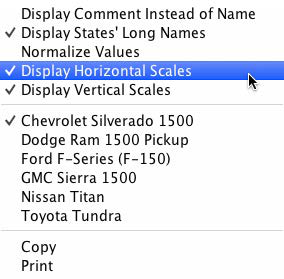
BayesiaLab offers a convenient way to see the relative position versus the segments. From the contextual menu, we can select Display Horizontal/Vertical Scales.
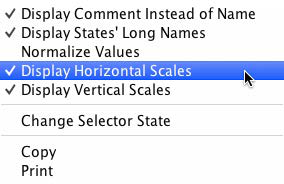
These scales show the range from the lowest to highest values. Additionally, a tick mark indicates the mean value of the respective attribute.
In the plot below, we show the Total Effect for Length of Time Vehicle Will Remain Solid/Durable for each segment. The intersection of the horizontal and vertical scales indicates the position of the Full-Size Pickup segment with regard to this variable.
This analysis can certainly help us to understand the general areas that are important for loyalty in the individual segments. However, it does not provide any insight into the specific opportunities for individual vehicle models. For this, we need to proceed to the next level of detail, i.e., the model level.
Multi-Quadrant Analysis (Segment ➔ Model)
During the earlier Multi-Quadrant Analysis, BayesiaLab generated one network file for each vehicle segment. We now open the network for the Full-Size Pickup, the focus of this study.
Although the structure of this segment-specific network is identical to that of the original network, all relationships between nodes, factors, and the target were re-estimated based on the subset of data corresponding to the Full-Size Pickup segment.
Relearning the Structure at the Market Level
As we move from the overall market into specific segments, and then models, we need to ask whether the structure learned at the market level will also hold true at the segment or model level.
In fact, we need to make a trade-off. We can retain the richer, more complex structure learned on the basis of the entire market, and simply reestimate the parameters. Alternatively, we can relearn the network structure on the much smaller dataset of the Full-Size Pickup segment. As opposed to the 71,200 cases for the entire market, we would then only have 2,003 observations [10] available for learning.
We hypothesize that the Full-Size Pickup segment has peculiarities that lead to structural differences versus the overall market. Consequently, we decide to relearn the network structure. The number of observations we have for this segment seems adequate to learn a reliable structure.
As before, we use the Augmented Markov Blanket algorithm: Learning > Supervised Learning > Augmented Markov Blanket.
[10] Count of unweighted observations.

We may find the resulting network a bit surprising as only a single arc is discovered, namely a connection between Affordable to Buy and Loyalty.
As we have not changed the default value, BayesiaLab used SC=1 for learning. Given the smaller amount of data available for this segment, we need to examine whether this is the appropriate value here.
Once again, we perform a Structural Coefficient Analysis: Tools > Cross Validation > Structural Coefficient Analysis.
As a result, we obtain the now-familiar scree plot, which suggests that SC=0.6 is a reasonable value.
We set the Structural Coefficient accordingly:
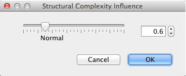
Once set, we proceed to relearning the network: Learning > Supervised Learning > Augmented Markov Blanket.
The resulting network now includes 7 factors. They appear fairly intuitive for this segment.
This is not to say that other factors do not matter. Rather, with the number of available observations, none other than the ones shown could be established with the given Structural Coefficient.
We now repeat the Target Mean Analysis: Analysis > Visual > Target Mean Analysis > Standard:
The resulting curves now show Loyalty as a function of the 7 factors in the network.
With the segment-specific network established, we can now proceed to the next level of detail, moving from Segment to Model.

For this purpose, we rerun the Multi-Quadrant Analysis and select Model as the Breakout Variable.
Furthermore, we must specify an output directory so we can subsequently analyze the model-specific networks.
Once again, we obtain a Quadrant Plot, now with Model as the selector.
As before, we can scroll through the individual states of the selector variable. By hovering over individual variables on the plot, we see the relative position of the models with respect to any factor.
The Display Horizontal/Vertical Scales command, which is available from the contextual menu of the Quadrant Plot, frames the range of competitors’ values.
Variations within the Realm of the Possible
This view is interesting on its own; however, we can more formally utilize this information. The position of each model on the attributes’ ranges allows us to compute the “gap to best/extreme level.” This will subsequently become very important as we look for ways to improve brand loyalty.
For instance, with regard to Factor 17, Fit Of Other Body Panels, the Dodge Ram achieves the highest rating, making it an appropriate target for competitors. If we were attempting to improve the rating of the GMC Sierra, the level of the Dodge Ram could be used as a target level.
Because this performance level has already been achieved, it is feasible and therefore realistic. This type of reference is precisely what we require for subsequent optimization. Without such a reference point, an optimization algorithm would happily recommend increasing the rating to a perfect 10, which is not helpful for practical purposes.
BayesiaLab can automatically extract the delta to highest and lowest levels for each factor. In this specific context, we call these deltas Variations. We will utilize these Variations as constraints for the optimization algorithm.
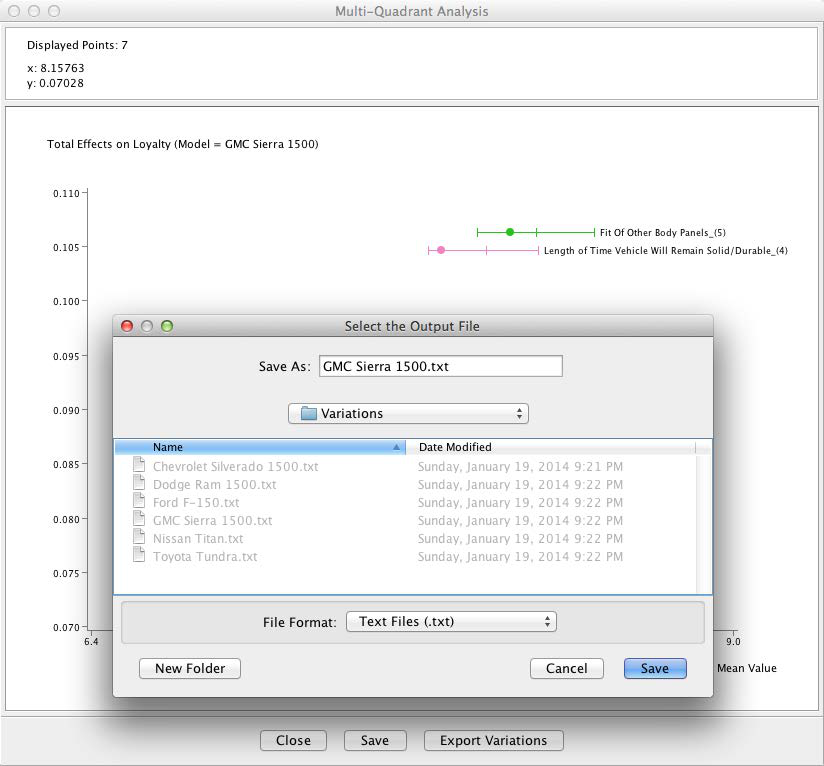
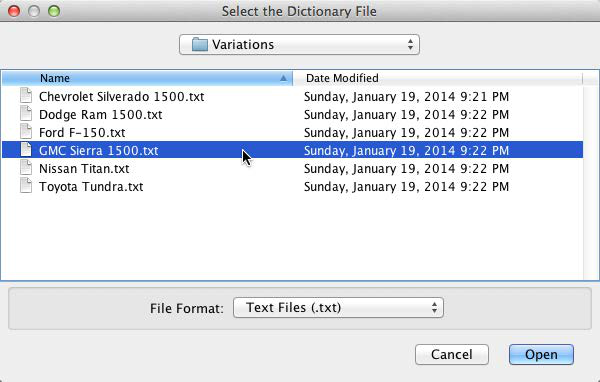
By clicking the Export Variations button, BayesiaLab saves the Variations for the currently selected model. For each model that we wish to optimize, we simply save this data as a text file.
Optimization
The Multi-Quadrant Analysis has generated new networks for each model, plus we have saved the associated Variations. Thus, we have all the components necessary for optimization. For the purpose of this tutorial, we will attempt to optimize the loyalty for the GMC Sierra.
To do so, we open the GMC Sierra-specific file generated by the most recent Multi-Quadrant Analysis.
Before proceeding to the optimization, we will briefly examine the Target Response Functions for the GMC Sierra, which we obtain via Target Mean Analysis (Standard).
As earlier, when we did this at the segment level, we also ran the Total Effects on Target report: Analysis > Report > Target Analysis > Total Effects on Target.
We obtain a report that shows the mean values of each factor, plus the corresponding Total Effects.
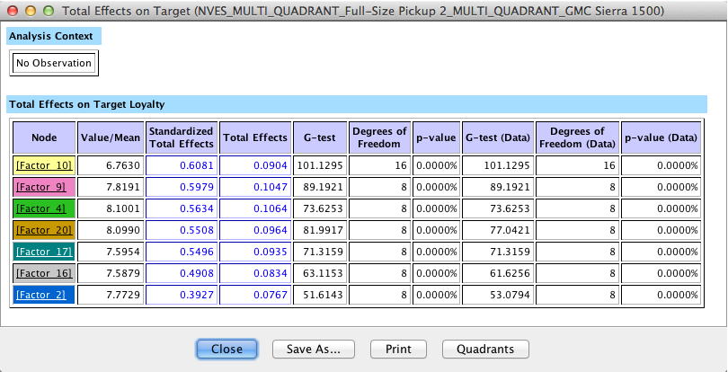
Here, the Quadrant Plot becomes very helpful as it shows both Value and Total Effects in a single plot.
There are many ways to interpret the above plot qualitatively. For instance, we may be tempted to look at Fit of Other Body Panels as the top driver and suggest focusing our efforts there. Also, we might say that Technical Innovations is fairly important, but has room for substantial improvement.
The challenge is to determine which combination of initiatives will yield the maximum improvement for loyalty, and what the new loyalty level would be.
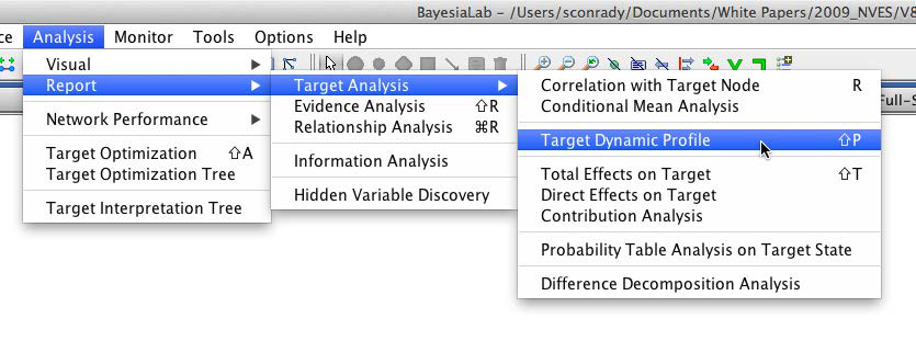
This brings us back to the central purpose of this study. We start optimization by selecting Analysis > Report > Target Analysis > Target Dynamic Profile.
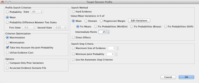
In the following window, we need to select several options that are critical in our search for optimal values. First, we are looking to maximize the mean of Loyalty (rather than, for instance, maximizing the probability of certain repurchase outcomes).
The checkbox Take Into Account Joint Probability is very important in our context. As we optimize, we need to bear in mind that loyalty is expressed as a probability. We might be tempted to look for a scenario in which we obtain 100% loyalty. However, the absolute number of units sold as a result of loyalty is critical from a business perspective. For instance, 100% loyalty within a niche of 100 customers generates fewer sales (i.e., 100 units) than an average loyalty of 50% among a larger group of 1,000 customers (i.e., 500 units).
So, pursuing an idealized state of perfect loyalty may be counterproductive as it might narrow the available customer base. This is where Joint Probability becomes an extremely helpful concept. By virtue of having learned a Bayesian network, we automatically have the joint probability of every conceivable combination of values of all nodes. This provides us with the ability to assess how far our optimized scenarios depart from the current reality. Considering this “stretch” beyond the status quo is central to our optimization approach.
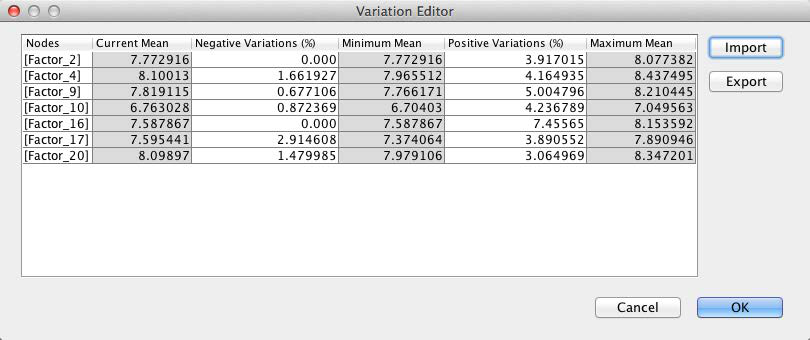
The second “reality check” relates to the variations, which we discussed earlier. By default, the Variation Editor is set to ±100%. This is what we see when we first open it.
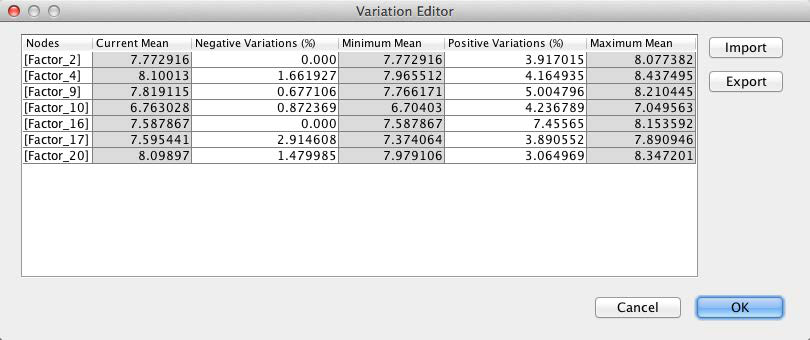
Now we re-introduce the variations we obtained earlier. By clicking Import, we can select the previously saved file with the Variations for the GMC Sierra.
With the Variations loaded, we see the ranges within which the optimization value can search for the optimal combination of values.
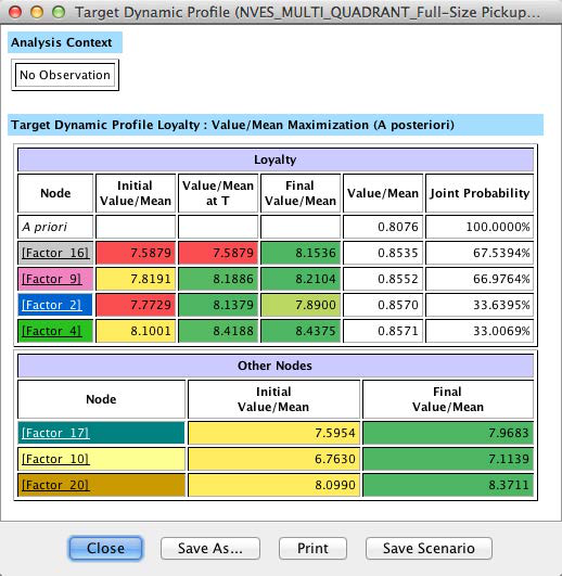
Clicking OK immediately starts the optimization routine. Given the small size of the network, the optimization report pops up within seconds.
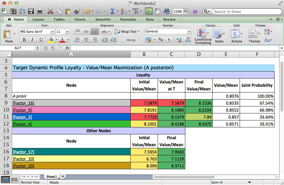
For a more detailed explanation, we save this report as an HTML file, which we can then open in Excel for further annotation. This file keeps all the formatting, including color-coding, of the on-screen report.
Recommendation for GMC Sierra 1500
The above report presents the results in a highly-condensed format. It will be helpful to dissect this table cell by cell. To properly interpret this table, it should be read line by line, top to bottom.
This table clearly spells out the top priorities for the GMC Sierra 1500. According to this simulation, achieving the new levels of the factors would lift loyalty from 0.80 to 0.85. For the GMC, this would translate into several thousand more customers returning to the brand.
For reference, the factor-to-manifest mapping is provided in the appendix below.
Given that the earlier Multi-Quadrant Analysis generated networks for all models in this segment, we could now repeat the optimization for any of the other models within minutes.
Summary
Bayesian networks and BayesiaLab make it possible to identify meaningful drivers from previously indistinguishable product ratings in survey data. On that basis, BayesiaLab can perform optimization and immediately establish priorities. With this approach, market researchers can quickly and transparently generate clear recommendations for decision-makers.
Appendix
Variables
Select Variables from the 2009 Strategic Vision New Vehicle Experience Survey (NVES)
- Combined Base Weight
- Door Handles - Exterior
- Fuel Efficiency
- Segment
- Badging (Exterior logos/identifiers)
- Emissions Control
- Make
- Exterior Color
- Front Seat Roominess
- Model
- Headlights Design
- 2nd row Seat Roominess
- Loyalty
- Taillights Design
- Ease of Front Seat Entry
- Safety Features
- Sunroof
- Ease of 2nd Row Seat Entry
- Front Visibility - Driver
- Interior Colors
- Comfort of Seatbelts
- Rear Visibility - Driver
- Interior Trim & Finish
- Support of Seats
- Braking
- Body Workmanship
- Passenger Seating Capacity
- Headlights Function
- Fit Of Doors
- Interior Storage Space
- Taillights Function
- Fit Of Other Body Panels
- Cargo Capacity
- Turn Signal Function
- Doors/Trunk/Hatch Shutting
- Cup Holders
- Airbags
- Wiper Performance (front/rear)
- Ease Of Trunk/Tailgate Operation
- Bumpers
- Quality Of Interior Materials
- Ease of Loading/Unloading Cargo
- Solid Vehicle Construction
- Instrument Cluster Gauges
- Front Seat Comfort
- Length of Time Vehicle Will Remain Solid/Durable
- Door Handles - Interior
- 2nd row Seat Comfort
- Interior Lighting
- Driver Seat Adjustability
- Freedom From Electrical Problems
- Quality of Seat Materials
- Passenger Seat Adjustability
- Ground Clearance
- Freedom From Squeaks And Rattles
- Driver Armrests
- Riding Comfort
- Freedom From Engine Noise
- Seating Versatility
- Maneuverability
- Freedom From Road Noise
- Seating Stowaway/Conversion
- Turning Radius
- Freedom From Wind Noise
- Placement Of Controls/Instruments
- Road Holding Ability
- Smoothness At Idle
- Electronic Display of Information
- Handling
- Smoothness Of Transmission
- Ease of Reading Controls/Instruments
- Steering Feedback
- Window Controls
- Usefulness of Glove Box
- Acceleration From Stop
- Wiper System Controls
- Usefulness of Trunk/Cargo Area
- Passing Capability
- Speed Control System
- Spare Tire
- Lines/Flow of the Vehicle
- Speakers
- Price Or Deal Offered
- Appearance Of Paint Job
- Ability to Control Sound Quality
- Future Trade-In Or Resale Value
- Size/Proportions
- Sound System Controls
- Warranty Coverage
- Side Mirrors
- CD Player
- Technical Innovations
- Appearance of Wheels & Rims
- Operation of HVAC Controls
- Level of Standard Equipment
- Appearance of Tires
- HVAC Vents
- Fuel Economy/Mileage
- Exterior Trim/Molding
- Defrost/Defog
- Economical to Own
List of Factors
- [Factor_0]: Door Handles - Interior, Ease of Reading Controls/Instruments, Electronic Display of Information, Instrument Cluster Gauges, Interior Lighting, Placement Of Controls/Instruments, Sunroof, Freedom From Engine Noise, Freedom From Road Noise
- [Factor_1]: Freedom From Squeaks And Rattles, Freedom From Wind Noise, Smoothness At Idle, Smoothness Of Transmission, Ease Of Trunk/Tailgate Operation, Ease of Loading/Unloading Cargo
- [Factor_2]: Spare Tire, Usefulness of Glove Box, Usefulness of Trunk/Cargo Area, Driver Armrests, Driver Seat Adjustability
- [Factor_3]: Passenger Seat Adjustability, Seating Stowaway/Conversion, Seating Versatility, Body Workmanship, Doors/Trunk/Hatch Shutting
- [Factor_4]: Fit Of Doors, Fit Of Other Body Panels, Wiper Performance (front/rear), Airbags, Bumpers
- [Factor_5]: Front Visibility - Driver, Rear Visibility - Driver, Safety Features, 2nd row Seat Roominess, Ease of 2nd Row Seat Entry
- [Factor_6]: Ease of Front Seat Entry, Front Seat Roominess, Passenger Seating Capacity, Appearance of Tires, Appearance of Wheels & Rims
- [Factor_7]: Badging (Exterior logos/identifiers), Door Handles - Exterior, Exterior Trim/Molding, Ground Clearance, Handling
- [Factor_8]: Riding Comfort, Road Holding Ability, Steering Feedback, Freedom From Electrical Problems
- [Factor_9]: Length of Time Vehicle Will Remain Solid/Durable, Prestige/Reputation of Mfr, Solid Vehicle Construction, Affordable to Buy
- [Factor_10]: Economical to Own, Future Trade-In Or Resale Value, Price Or Deal Offered, Appearance Of Paint Job
- [Factor_11]: Lines/Flow of the Vehicle, Side Mirrors, Size/Proportions, Interior Colors
- [Factor_12]: Interior Trim & Finish, Quality Of Interior Materials, Quality of Seat Materials, Braking
- [Factor_13]: Headlights Function, Taillights Function, Turn Signal Function, 2nd row Seat Comfort
- [Factor_14]: Comfort of Seatbelts, Front Seat Comfort, Support of Seats, Ability to Control Sound Quality
- [Factor_15]: CD Player, Sound System Controls, Speakers, Cargo Capacity
- [Factor_16]: Cup Holders, Interior Storage Space, Level of Standard Equipment
- [Factor_17]: Technical Innovations, Warranty Coverage, Exterior Color
- [Factor_18]: Headlights Design, Taillights Design, Emissions Control
- [Factor_19]: Fuel Economy/Mileage, Fuel Efficiency, Speed Control System
- [Factor_20]: Window Controls, Wiper System Controls, Defrost/Defog
- [Factor_21]: HVAC Vents, Operation of HVAC Controls
- [Factor_22]: Maneuverability, Turning Radius
- [Factor_23]: Acceleration From Stop, Passing Capability