Case Study: Vehicle Size, Weight, and Injury Risk
Introduction
Objective
This paper aims to illustrate how Bayesian networks and BayesiaLab can help overcome certain limitations of traditional statistical methods in high-dimensional problem domains. We consider the vehicle safety discussion in the recent Final Rule on future CAFE standards issued by the Environmental Protection Agency (EPA) and the National Highway Traffic Safety Administration (NHTSA) to be an ideal topic for our demonstration purposes.
When we reference the EPA/NHTSA Final Rule, we are specifically referring to the version of the document that was signed on August 28, 2012, and subsequently submitted to the Federal Register. However, when discussing the overall rationale presented in the Final Rule, we also implicitly include all the supporting studies that informed it. The Corporate Average Fuel Economy (CAFE) regulation was enacted by the U.S. Congress in 1975 with the goal of improving the average fuel economy of passenger cars and light trucks.
This paper focuses on technique rather than the subject matter itself, but our findings will undoubtedly yield new insights. We do not intend to challenge the conclusions of the EPA/NHTSA Final Rule. Instead, we aim to examine the overall problem domain independently while considering the rationale outlined in the Final Rule. Rather than simply replicating existing analyses with different tools, we will incorporate a broader set of variables and employ alternative methods to provide a complementary perspective on certain aspects of this issue. By moving beyond the traditional parametric methods used in EPA/NHTSA studies, we intend to demonstrate how Bayesian networks can serve as a robust framework for forecasting the impacts of regulatory interventions. Ultimately, our goal is to utilize Bayesian networks to evaluate the consequences of actions that have yet to be taken.
We will restate several original research questions to better align with our explanatory goals. While the EPA/NHTSA required a macro view of this domain, focusing on societal costs and benefits, we believe that Bayesian networks are particularly effective for understanding high-dimensional dynamics at a micro level. Therefore, we will examine this area with greater detail by incorporating additional accident attributes and using finer measurement scales.
For the sake of clarity, we will also limit our study to a more narrowly defined context, specifically vehicle-to-vehicle collisions rather than all types of motor vehicle accidents. It is important to emphasize that our analysis will focus solely on vehicle safety. We will not address any of the environmental justifications presented in the EPA/NHTSA Final Rule. Thus, our focus will be on a small segment of the overall problem domain.
This paper demonstrates a typical research workflow by presenting a sequence of alternating questions and answers. Throughout this discussion, we will gradually introduce various concepts specific to Bayesian networks, addressing each topic as it arises. In the initial chapters, we focus on providing extensive detail, including step-by-step instructions and numerous screenshots for using BayesiaLab. As we progress to later chapters, we will begin to simplify some of the technical aspects to emphasize the broader perspective of Bayesian networks as a powerful framework for reasoning.
Background
In October 2012, the Environmental Protection Agency (EPA) and the National Highway Traffic Safety Administration (NHTSA) issued the Final Rule, “2017 and Later Model Year Light-Duty Vehicle Greenhouse Gas Emissions and Corporate Average Fuel Economy Standards.”
One of the most important concerns in the Final Rule was its potential impact on vehicle safety. This should not be surprising as it is a commonly held notion that larger and heavier vehicles, which are less fuel-efficient, are generally safer in accidents. This belief is supported by the principle of conservation of linear momentum and Newton’s well-known laws of motion. In collisions of two objects of different mass, the deceleration force acting on the heavier object is smaller. Secondly, larger vehicles typically have longer crumple zones that extend the time over which the velocity change occurs, thus reducing the deceleration. Vehicle manufacturers and independent organizations have observed this many times in crash tests under controlled laboratory conditions.
It is also known that vehicle size and weight are key factors for fuel economy (please note that “Weight” and “mass” are used interchangeably throughout this paper). More specifically, the energy required to propel a vehicle over any given distance is a linear function of the vehicle’s frontal area and mass. Thus, a reduction in mass directly translates into a reduced energy requirement, i.e. lower fuel consumption.
Therefore, at least in theory, a conflict of objectives arises between vehicle safety and fuel economy. The question is, what does the real world look like? Are smaller, lighter cars really putting passengers at substantially greater risk of injury or death? One could hypothesize that so many other factors influence the probability and severity of injuries, including highly advanced restraint systems, that vehicle size may ultimately not determine life or death.
Given that the government, both at the state and the federal level, has collected records regarding hundreds of thousands of accidents over decades, one would imagine that modern data analysis can produce an in-depth understanding of injury risk in real-world vehicle crashes.
This is precisely what EPA and NHTSA did in order to estimate the societal costs and benefits of the proposed new CAFE rule. In fact, a large portion of the 1994-page Final Rule is devoted to discussing vehicle safety. Based on their technical and statistical analyses, they conclude that there is a safety-neutral compliance path with the new CAFE standards that includes mass reduction (we refer to the version of the document signed on August 28, 2012, which was submitted to the Federal Register. Page numbers refer to this version only).
General Considerations
To provide motivation and context for our proposed workflow, we will briefly discuss a number of initial thoughts regarding the EPA/NHTSA Final Rule. As an introduction to the technical discussion, we will first bring up a number of general considerations about the problem domain that will influence our approach.
Active Versus Passive Safety
The EPA/NHTSA studies have used “fatalities by estimated vehicle miles traveled (VMT)” as the principal dependent variable. This measure thus reflects all contributing as well as mitigating factors with regard to fatality risk. This includes human characteristics and behavior, environmental conditions, and vehicle characteristics, and behavior (e.g. small passenger car with ABS and ESP). In fact, the fatality risk is a function of one’s own attributes as well as the attributes of any other participant in the accident. In order to model the impact of vehicle weight reduction at the society-level, one would naturally have to take all of the above into account.
As opposed to a society-level analysis, we are approaching this domain more narrowly by looking at the risk of injury only as a function of vehicle characteristics and accident attributes. We believe that this approach helps to isolate vehicle crashworthiness, i.e. a vehicle’s passive safety performance, as opposed to performing a joint analysis of crash propensity and crashworthiness. This implies that we omit the potential relevance of vehicle attributes and occupant characteristics with regard to preventing an accident, i.e. active safety performance. It would be quite reasonable to include the role of vehicle weight in the context of active safety. For instance, the braking distance of a vehicle is, among other things, a function of vehicle mass. Similarly, occupant characteristics most certainly affect the probability of accidents, with younger drivers being a well-known high-risk group.
As a result of drivers’ characteristics and vehicles’ behavior, at least a portion of victims (and their vehicles) “self-select” themselves through their actions to “participate” in an accident. Speaking in epidemiological terms, our study may thus be subject to a self-selection bias. This would indeed be an issue that would have to be addressed for society-level inference. However, this potential self-selection bias should not interfere with our demonstration of the workflow while exclusively focusing on passive safety performance.
Dependent Variable
The EPA/NHTSA studies use a binary response variable, i.e. fatal vs. non-fatal, in order to measure accident outcomes. In the narrower context of our study, we believe that a binary response variable may not be comprehensive enough to characterize the passive safety performance of a vehicle.
Also, survival is not only a function of the passive safety performance of a vehicle during an accident, but it is also influenced by the quality of the medical care provided to the accident victim after the accident.
While it is a widely held belief among experts that vehicle safety has much improved over the last decade, the recent study by Glance et al. (2012) reports that, given the same injury level, there has also been a significant reduction in mortality of trauma patients since 2002.
“In-hospital mortality and major complications for adult trauma patients admitted to level I or level II trauma centers declined by 30% between 2000 and 2009. After stratifying patients by injury severity, the mortality rate for patients presenting with moderate or severe injuries declined by 40% to 50%, whereas mortality rates remained unchanged in patients with the least severe or the most severe injuries.”
Given that the fatality data that was used to inform the EPA/NHTSA Final Rule was collected between 2002 and 2008, we speculate that identical injuries could have had different outcomes, i.e. fatal versus non-fatal, as a function of the year when the injury occurred. Thus, we find it important to use an outcome variable that characterizes the severity of injuries sustained during the accident, as opposed to only counting fatalities.
Covariates
Similar to the binary fatal/non-fatal classification, other key variables in the EPA/NHTSA studies are also binned into two states, e.g., two weight classes While the discretization of variables will also become necessary in our approach with Bayesian networks, we hypothesize that using two bins may be too “coarse” as a starting point. By using two intervals only, we would implicitly make the assumption of linearity in estimating the effect of vehicle weight on the dependent variable.
Furthermore, we speculate that a number of potentially relevant covariates can be added to provide a richer description of the accident dynamics. For instance, in a collision between two vehicles, we presume the angle of impact to be relevant, e.g. whether an accident is a frontal collision or a side impact. Also, specifically for two-vehicle collisions, we consider that the mass of both vehicles is important, as opposed to measuring this variable for one vehicle only. We will attempt to address these points with our selection of data sources and variables.
Consumer Response
The “law of unintended consequences” has become an idiomatic warning that an intervention in a complex system often creates unanticipated and undesirable outcomes. One such unintended consequence might be the consumers’ response to the new CAFE rule.
The EPA/NHTSA Final Rule notes that all statistical models suggest a mass reduction in small cars would be harmful or, at best, close to neutral and that the consumer choice behavior given price increases is unknown. Also, the EPA/NHTSA Final Rule has put great emphasis on preventing vehicle manufacturers from “downsizing” vehicles as a result of the CAFE rule: “in the agencies’ judgment, footprint-based standards [for manufacturers] discourage vehicle downsizing that might compromise occupant protection.” (EPA Final Rule, p. 214).
However, the EPA/NHTSA Final Rule does not provide an impact assessment with regard to future consumer choices in response to the new standards. Given that the Final Rule states that vehicle prices for consumers will rise significantly, “between $1,461 and $1,616 per vehicle in MY 2025” (EPA Final Rule, p. 123) as a direct consequence of the CAFE rule, one can reasonably speculate that consumers might downsize their vehicles.
Rather, the Final Rule states: “Because the agencies have not yet developed sufficient confidence in their vehicle choice modeling efforts, we believe it is premature to use them in this rulemaking.” (EPA Final Rule, p. 310). We speculate that this may limit one’s ability to draw conclusions with regard to the overall societal cost.
Unfortunately, we currently lack the appropriate data to build a consumer response model that would address this question within our framework. However, in terms of the methodology, we have presented a vehicle choice modeling approach in our white paper, Modeling Vehicle Choice and Simulating Market Share.
Technical Considerations
Assumption of Functional Forms
Given the familiar laws of physics that are applicable to collisions, one could hypothesize about certain functional forms for modeling the mechanisms that cause injuries of vehicle passengers. However, a priori, we cannot know whether any such assumptions are justified. Because this is a common challenge in many parametric statistical analyses, one would typically require a discussion regarding the choice of functional form, e.g. justifying the assumption of linearity.
We are not in a position to reexamine the choice of functional forms in the EPA/NHTSA studies. However, our proposed approach, learning Bayesian networks with BayesiaLab, has the advantage that no specification of any functional forms is required at all. Rather, BayesiaLab’s knowledge discovery algorithms use information-theoretic measures to search for any kind of probabilistic relationships between variables. As we will demonstrate later, we can capture the relationship between injury severity and angle of impact, which is clearly nonlinear.
Interactions and Collinearity
All of the studies supporting the EPA/NHTSA Final Rule use a broad set of control variables in their regression models. However, none of the studies use any interaction effects between these covariates. As such, an assumption is implicitly made that the covariates are all independent. However, examining the relationships between the covariates reveals that strong correlations do indeed exist, which violates the assumption of independence. In fact, collinearity is highlighted numerous times, e.g. “NHTSA considered the near multicollinearity of mass and footprint to be a major issue in the 2010 report and voiced concern about inaccurately estimated regression coefficients.” (Kahane, p. xi).
The nature of learning a Bayesian network does automatically take into account a multitude of potential relationships between all variables and can even include collinear relationships without a problem. We will see that countless relevant interactions between covariates exist, which are essential to capture the dynamics of the domain.
Causality
This last point is perhaps the most challenging one among the technical issues. The EPA/NHTSA studies use statistical models for purposes of causal inference. Statistical (or observational) inference, as in “given that we observe,” is not the same as causal inference, as in “given that we do.” Only under strict conditions, and with many additional assumptions, can we move from the former to the latter.9 Admittedly, causal inference from observational data is challenging and can be controversial. All the more it is important to clearly state the assumptions and why they might be justified.
With Bayesian networks we want to present a framework that allows researchers to explore this domain in a “causally correct” way, i.e., allowing, with the help of human domain knowledge, to disentangle “statistical correlation” and “causal effects.”
Exploratory Analysis
Data Overview
In order to better understand the nature of accidents, the National Automotive Sampling System (NASS) Crashworthiness Data System (CDS) was established as a nationwide crash data collection program sponsored by the U.S. Department of Transportation. The National Center for Statistics and Analysis (NCSA), part of the National Highway Traffic Safety Administration (NHTSA), started the data collection for the NASS program in 1979. Data collection is accomplished at 24 geographic sites, called Primary Sampling Units (PSUs). These data are weighted to represent all police-reported motor vehicle crashes occurring in the USA during the year involving passenger cars, light trucks, and vans that were towed due to damage. All data are available publicly from NHTSA’s FTP server.10
Data Set for Study
We use the following subset of files from the 11-file dataset published by NHTSA (ftp://ftp.nhtsa.dot.gov/NASS):
- ACC: Accident Record (accident.sas7bdat)
- GV: General Vehicle Record (gv.sas7bdat)
- OA: Occupant Assessment Record (oa.sas7bdat)
- VE: Exterior Vehicle Record (ve.sas7bdat)
We have joined the records of these tables via their unique identifiers and then concatenated all files from 1995 through 2011 into a single table. This table contains records regarding approximately 200,000 occupants of 100,000 vehicles involved in 37,000 accidents. Each record contains more than 400 variables, although there is a substantial amount of missing values. The comprehensive nature of this dataset is ideal for our exploration of the interactions of crash-related variables and their ultimate impact on passenger safety.
Notation
- All variable names/labels follow the format “DatasetAbbreviation_VariableName”, e.g. GV_SPLIMIT for the variable from the dataset General Vehicle Record.
- All variable and node names are italicized.
- Names of BayesiaLab-specific features and functions are capitalized and shown in bold type.
Data Filters and Variable Selection
To start with our exploration of this problem domain, we narrow our focus by selecting subsets of variables and records:
- We restrict our analysis to horizontal vehicle-to-vehicle collisions, with the vehicle under study being MY2000 or later. We consider MY2000 a reasonable cutoff point, as by then second-generation airbags were mandatory for all passenger vehicles. In this context, we only examine the condition of the driver. Also, we exclude collisions involving large trucks (Gross Vehicle Weight Rating (GVWR) > 10,000 lbs.) and motorcycles. For data consistency purposes, we filter out unusual and very rare accident types, e.g. accidents with principal deformation to the underside of the vehicle. We apply these filters primarily for expositional simplicity. However, we do recognize that this limits our ability to broadly generalize the findings.
- However, no records are excluded solely due to missing values. BayesiaLab offers advanced missing values processing techniques, which we can leverage here. This is an important point as the vast majority of records contain some missing values. In fact, if we applied a traditional casewise/listwise deletion, most records would be eliminated from the database.
- Furthermore, many of the 400+ variables provide a level of detail that far exceeds the scope of this paper. Thus, we limit our initial selection to 19 variables that appear a priori relevant and are generally in line with the variables studied in the EPA/NHTSA research.
- In addition to the variables defined in the NASS/CDS database, we introduce GV_FOOTPRINT as a variable that captures vehicle footprint.13 This new variable is computed as the product of VE_WHEELBAS (Wheelbase) and VE_ORIGAVTW (Average Track Width), which are recorded in the original database (“Footprint is defined as a vehicle’s wheelbase multiplied by its average track width - in other words, the area enclosed by the points at which the wheels meet the ground.” Final Rule, p. 69).
The following table summarizes the variables included in our study.
| Variable Name | Long Name | Units/States | Comment |
|---|---|---|---|
| GV_CURBWGT | Vehicle Curb Weight | kg | |
| GV_DVLAT | Lateral Component of Delta V | km/h | |
| GV_DVLONG | Longitudinal Component of Delta V | km/h | |
| GV_ENERGY | Energy Absorption | J | |
| GV_FOOTPRINT | Vehicle Footprint | m2 | calculated as WHEELBAS x ORIGAVTW |
| GV_LANES | Number of Lanes | count | |
| GV_MODELYR | Vehicle Model Year | year | |
| GV_OTVEHWGT | Weight Of The Other Vehicle | kg | |
| GV_SPLIMIT | Speed Limit | mph | converted into U.S. customary units |
| GV_WGTCDTR | Truck Weight Code | missing = Passenger Vehicle | |
| 6,000 and less | |||
| 6,001-10,000 | |||
| OA_AGE | Age of Occupant | years | |
| OA_BAGDEPLY | Air Bag System Deployed | Nondeployed | |
| Bag Deployed | |||
| OA_HEIGHT | Height of Occupant | cm | |
| OA_MAIS | Maximum Known Occupant AIS | Not Injured | AIS Probability of Death |
| Minor Injury | 0% | ||
| Moderate Injury | 1-2% | ||
| Serious Injury | 8-10% | ||
| Severe Injury | 5-50% | ||
| Critical Injury | 5-50% | ||
| Maximum Injury | 100% (Unsurvivable) | ||
| Unknown | Missing Value | ||
| OA_MANUSE | Manual Belt System Use | Used | |
| Not Used | |||
| OA_SEX | Occupant’s Sex | Male | |
| Female | |||
| OA_WEIGHT | Occupant’s Weight | kg | |
| VE_GAD1 | Deformation Location (Highest) | Left | |
| Front | |||
| Rear | |||
| Right | |||
| VE_PDOF_TR | Clock Direction for Principal Direction of Force (Highest) | Degrees | Transformed variable, rotated 135 degrees counterclockwise |
OA_MAIS (Maximum Known Occupant AIS)
The outcome variable represents the . “AIS” stands for “Abbreviated Injury Scale.” The Abbreviated Injury Scale is an anatomically-based, consensus-derived global severity scoring system that classifies each injury by body region according to its relative importance on a 6-point ordinal scale (1=minor and 6=maximal).
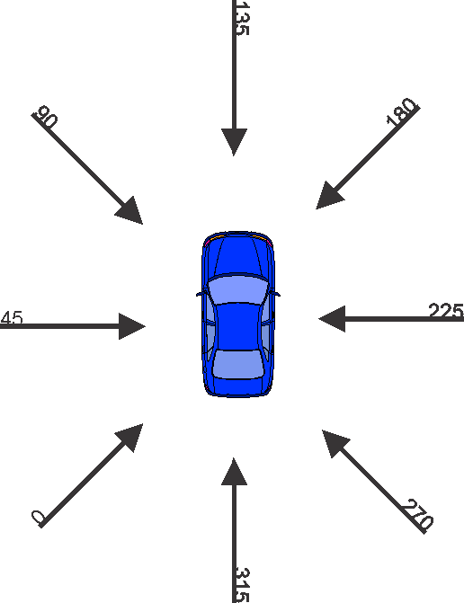
Coordinate System for Variable PDOF1 (Principal Direction of Force)
Most of the variables’ scales and units are self-explanatory, perhaps with the exception of GV_PDOF1 (Principal Direction of Force). This variable records the direction of the highest force acting on the vehicle during the accident. A frontal collision, i.e. in the direction of travel from the perspective of the vehicle under study, would imply PDOF1=0. Conversely, a rear impact would mean PDOF1=180, etc.
Given the requirements of data discretization as part of the data import process (see next chapter), we rotate the coordinate system by 135 degrees counterclockwise. The values in this new coordinate system are recorded in the transformed variable . This rotation prevents that frequently occurring, similar values (e.g. frontal collisions at 355 degrees, 0 degrees, and 5 degrees on the original scale) are split into different bins due to the natural break at 0 degrees.
To make it easier to interpret the values of the transformed variable , we briefly illustrate our new coordinate system. For instance, a VE_PDOF_TR=45 now means that the vehicle under study collided on the driver’s side and that the impact was perpendicular to the direction of travel. A 135 degrees impact represents a direct frontal collision, e.g. with oncoming traffic. Conversely, a rear-end collision is represented by a 315 degrees angle.

This coordinate system may become more intuitive to understand when it is viewed in quadrant form, in a clockwise direction:
- 0 degrees-90 degrees: Impact from left
- 90 degrees-180 degrees: Frontal impact
- 180 degrees-270 degrees: Impact from right
- 270 degrees-360 degrees: Rear impact
To confirm the plausibility of this transformed variable, we can plot GV_DVLAT and GV_DVLONG as a function of VE_PDOF_TR. We would anticipate that a full frontal impact, i.e. _VE_PDOF_TR=135, would be associated with the highest decrease in velocity, i.e. GV_DVLONG≪0. At the same time, we would expect the lateral Delta V to be near zero, i.e. GV_DVLAT≈0. This is indeed what the following plots confirm. They also illustrate the respective signs of Delta V as a function of the impact angle.
In BayesiaLab, we can quickly create scatterplots by selecting Menus > Data > Chart.
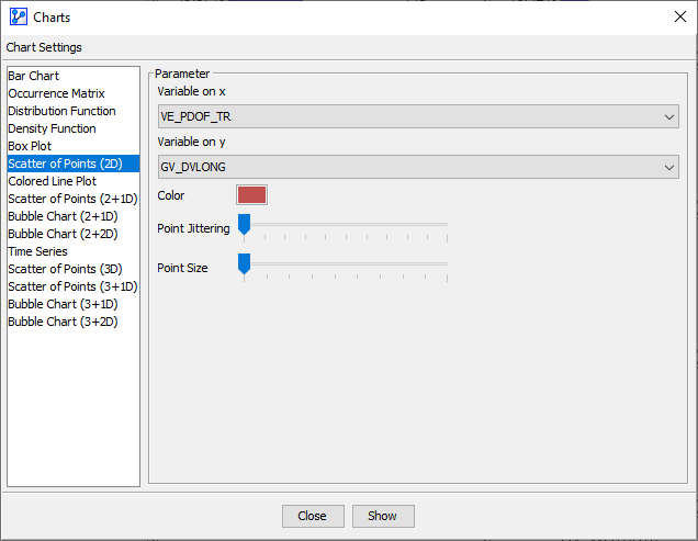
Upon selecting the respective variables for display, BayesiaLab produces the corresponding plots.


Data Import
The first step in our process towards creating a Bayesian network is importing the raw data into BayesiaLab. Please see Open Data Source (Data Import Wizard) for details of the data import workflow.
However, we should note that we adjust some of the bins that were found by BayesiaLab’s automatic discretization algorithms, so they reflect typical conventions regarding this domain. For instance, if the discretization algorithm proposed a bin threshold of 54.5 for GV_SPLIMIT, we would change this threshold to 55 (mph) in order to be consistent with our common understanding of speed limits.
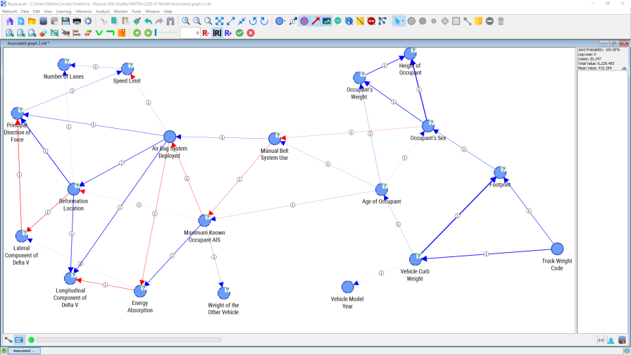
Upon completion of the import process, we obtain an initially unconnected network, which is shown below. All variables are now represented by nodes, one of the core building blocks in a Bayesian network. A node can stand for any variable of interest. Discretized nodes are shown with a dashed outline, whereas solid outlines indicate discrete variables, i.e. variables with either categorical or discrete numerical values. Once the variables appear in this new form in a graph, we will exclusively refer to them as nodes.

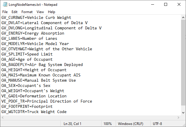
At this point, it is practical to add Long Node Names to the Node Names that are displayed under each node by default. In BayesiaLab, Long Node Names are typically used for more descriptive titles, which can be turned on or off, depending on the desired view of the graph. Here, we associate a dictionary with Long Node Names, while the more compact variable names of the original dataset remain as Node Names (to maintain a compact presentation, we will typically use the original variable name when referencing a particular node).
The syntax for this association is rather straightforward: we simply define a text file that includes one Node Name per line. Each Node Name is followed by the equal sign (“=”), or alternatively TAB or SPACE, and then by the long variable description, which will serve as the Long Node Name.
This file can then be loaded into BayesiaLab via Menus > Data > Associate Dictionary > Node > Long Names. Then, after highlighting all nodes, we can select Node Contextual Menu > Properties > Rendering Properties > Show Long Name. Checking the Show Long Name box and clicking OK, brings up the Long Names in the Graph Panel.

Long Node Names can be displayed either for all nodes or only for selected ones. Given the sometimes cryptic nature of the original variable names, we will keep the more self-explanatory Long Node Names turned on for most analyses. Also, we can separately turn on the Long Names for the Monitor Panel: Monitor Panel Contextual Menu > Show > Long Name of Nodes.
Initial Review
Upon data import, it is good practice to review the probability distributions of all nodes. The best way to get a complete overview is to switch to Validation Mode (F5), select all nodes (Ctrl+A), and then double-click on any one of them. This brings up the Monitors for each node within the Monitor Panel.

Each Monitor contains a histogram representing the marginal probability distributions of the states of its associated node. This allows us to review the distributions and compare them with our own domain understanding. For instance, the gender mix, OA_SEX, is approximately at the expected uniform level, and other nodes appear to have reasonable distributions, too.
Distance Mapping
Going beyond these basic statistics of individual nodes, we can employ a number of visualization techniques offered by BayesiaLab. Our starting point is Distance Mapping based on Mutual Information: Menus > View > Layout > Distance Mapping > Mutual Information. As the name of this layout algorithm implies, the generated layout is determined by the Mutual Information between each pair of nodes.
By invoking the Distance Mapping function, Menus > View > Layout > Distance Mapping > Mutual Information, BayesiaLab presents the distance between any pair of nodes inversely proportional to their Mutual Information.
Among all nodes in our example, there appear to be several clusters that can be intuitively interpreted. Principal Direction of Force and Deformation Location, in the above graph, reflect impact angle and deformation location, two geometrically connected metrics. Footprint, Vehicle Curb Weight, and Truck Weight Code are closely related to each other and to the overarching concept of vehicle size. Quite literally, knowing the state of a given node reduces our uncertainty regarding the states of the nearby nodes.
Unsupervised Learning
When exploring a new domain, we usually recommend performing Unsupervised Learning on the newly imported database. This is also the case here, even though our principal objective is targeted learning, for which Supervised Learning will later be the main tool. Menus > Learning > Unsupervised Structural Learning > EQ initiates the EQ algorithm, which is suitable for the initial review of the database.
In its raw form, the crossing arcs make this network somewhat tricky to read. BayesiaLab has a number of layout algorithms that can quickly disentangle such a network and produce a much more user-friendly format. We select Menus > View > Automatic Layout or alternatively use the shortcut P.
Now we can visually review the learned network structure and compare it to our own domain knowledge. This allows us to do a “sanity check” of the database and the variables, and it may highlight any inconsistencies.
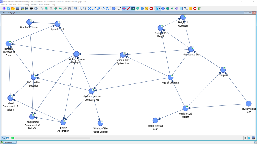
Indeed, in our first learning attempt, we immediately find 34 arcs between the 19 variables included in the model, so interactions appear to be manifold.
Although it is tempting, we must not interpret the arc directions as causal directions. What we see here, by default, are merely statistical associations, not causal relations. We would have to present a significant amount of theory to explain why Bayesian networks always must have directed arcs. However, this goes beyond the scope of this presentation. Rather, we refer to the literature listed in the references and our other white papers.
Mapping
Beyond qualitatively inspecting the network structure, BayesiaLab allows us to visualize the quantitative part of this network. To do this, we first need to switch to the Validation Mode F5. In Validation Mode, we start the Mapping function: Menus > Analysis > Visual > Mapping
The Mapping window opens up and presents a new view of the graph.
The Mapping window features drop-down menus for Node Analysis and Arc Analysis. However, we are only interested in Arc Analysis at this time and select Pearson Correlation as the metric to be displayed.
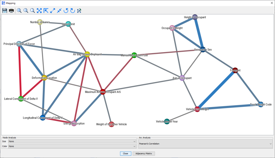
The thickness of the arcs, beyond a fixed minimum size, is now proportional to the Pearson Correlation between the nodes. Also, the blue and red colors indicate positive and negative correlations respectively.
BayesiaLab can also visualize the same properties in a slightly different format. This is available via Menus > Analysis > Visual > Overall > Arc > Pearson Correlation.
Here, too, the arc thickness is proportional to Pearson Correlation. Additionally, callouts indicate that further information can be displayed. We opt to display this numerical information via Menus > View > Show Arc Comments.
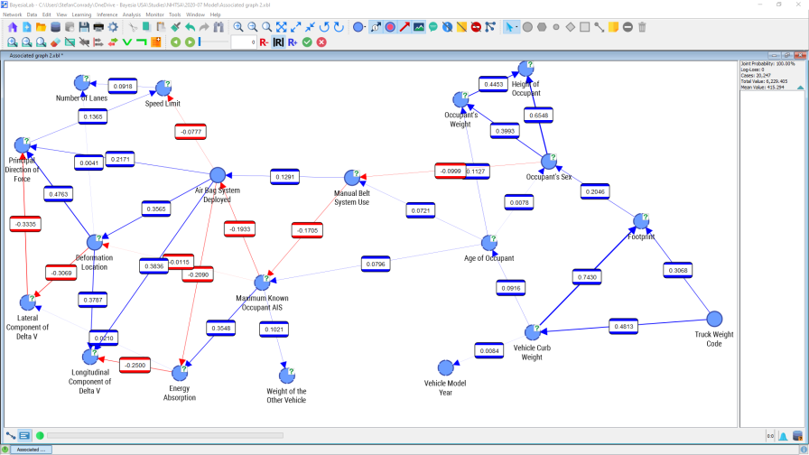
The multitude of numbers presented in this graph can still be overwhelming. We may wish to “tune out” weaker connections to focus on the more important ones. The slider control within the menu bar allows us to interactively change the threshold below which connections should be excluded from display.
In this setting, only nodes are shown that are connected with an absolute correlation coefficient of 0.34 or higher. The remaining nodes and arcs, below that threshold, are grayed out.
There are a number of nodes that stand out as highly correlated, in particular Vehicle Curb Weight, Truck Weight Code, and Footprint. This is plausible as these nodes can be understood as proxies for overall vehicle size. Strong relationships also exist between Height of Occupant, Occupant’s Weight, and Occupant’s Sex, which is consistent with our general knowledge that men, on average, are taller and heavier than women.
Note that BayesiaLab can compute Pearson Correlation for any pair of nodes with ordered states, regardless of whether they are numerical or categorical (e.g. Monday, Tuesday, etc.). However, the computed values are only meaningful if a linear relationship can be assumed. For some of the node pairs shown above, this may not be an unreasonable hypothesis. In the case of Deformation Location and Principal Direction of Force it would not be sensible to interpret the relationship as linear. Rather, the computed correlation is purely an artifact of the random ordering of states of Deformation Location. However, we will see in the next section that strong (albeit nonlinear) links do exist between these variables.
Mutual Information
An alternative perspective on the relationships can be provided by displaying Arc’s Mutual Information, which is a valid measure regardless of variable type, i.e. including the relationships between (not-ordered) categorical and numerical variables: Menus > Analysis > Visual > Overall > Arc > Mutual Information.
As before, we can bring up the numerical information by selecting Menus > View > Show Arc Comments.

Mutual Information I(X,Y) measures how much (on average) the observation of a random variable tells us about the uncertainty of X, i.e. by how much the entropy of X is reduced if we have information on Y. Mutual Information is a symmetric metric, which reflects the uncertainty reduction of X by knowing Y as well as of Y by knowing X.
We can once again use the slider in the menu bar to adjust the threshold for the display of arcs. Moving the slider towards the right, we gradually filter out arcs that fall below the selected threshold.

Focusing on one particular relationship, we can see that knowing the value of Deformation Location on average reduces the uncertainty of the value of Principal Direction of Force by 0.8120 bits.
Conversely, knowing Principal Direction of Force reduces the uncertainty of Deformation Location by 0.8120 because Mutual Information is a symmetric metric.
Bayesian Network Properties
It is necessary to emphasize that, despite the visual nature of a Bayesian network, it is not a visualization of data. Rather, it is the structure that is visualized. So, what we see is the model, not the data. The Bayesian network is meant to be a generalization of the underlying data, rather than a “bit-perfect” replica of the data. Theoretically, and at a huge computational cost, a fully-connected Bayesian network can produce a perfect fit. However, that would bring us back to nothing more than the raw data, instead of generating an interpretable abstraction of the data.
Omnidirectional Inference
Any network that we see here is a fully specified and estimated model that can be used for inference. A particularly important property is what we call “omnidirectional inference.” While traditional statistical models usually contain one dependent and many independent variables, that distinction is not necessary for a Bayesian network. In fact, all variables can be treated equivalently, which is particularly interesting for exploratory research.
To gain familiarity with all the interactions learned from the data, we will experiment with omnidirectional inference and run various exploratory queries on different subsets of the model.
Example 1: Number of Lanes, Deformation Location, and Speed Limit
In Validation Mode, double-clicking on an individual node, or on a selected set of nodes, brings up the corresponding Monitors on the righthand-side Monitor Panel. Conversely, double-clicking again would remove them.

For instance, we show the Monitors for Number of Lanes, Speed Limit, and Deformation Location. Small histograms will show us the marginal distributions of those variables.
We can see that of all accidents 38.96% occur on roads with 3 or 4 lanes, or that 17.23% happen in areas with speed limits greater than 50 mph.
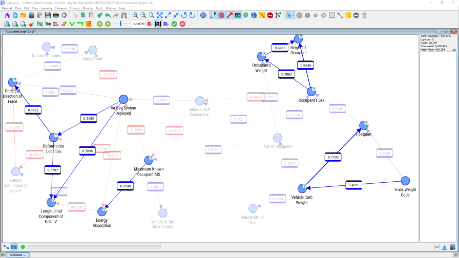
We might now want to ask the question, “what is the distribution of impact angles for accidents that happen on roads with more than 4 lanes?” We can use the network to answer this query by “setting evidence” via the Monitor for Number of Lanes. In BayesiaLab, this simply requires a double-click on the “>4” bar of this Monitor. Upon setting the evidence, the Number of Lanes>4 bar turns green, and we can now read the posterior probability distributions of the other nodes.
We see, for instance, that the share of left-side collisions has dropped from 16.27% to 9.22%. However, we can observe another change. Given that we are focusing on roads with 5 or more lanes, now only 8.69% have a speed limit of 30 mph or below. In the marginal distribution, this share was 21.54%. The little gray arrows indicate the amount of change versus the previous distribution.
The Maximum Variation of Probabilities can be displayed by selecting Monitor > Highlight Maximum Probability Variations.
It is now obvious that one piece of evidence, i.e. setting Number of Lanes>4, has generated multiple updates to other variables’ distributions as if we had multiple dependent variables. In fact, all variables throughout the network were updated, but we only see the changes in distributions of those nodes that are currently shown in the Monitor Panel.
We now set the second piece of evidence, Speed Limit>50.
As a result, we see a big change in Deformation Location=Rear, i.e. rear impacts; their probability jumps from 9.10% to 17.29%. Again, this should not be surprising as roads with more than 4 lanes and with speed limits of 50 mph or higher are typically highways with fewer intersections. Presumably, less cross-traffic would cause fewer side impacts.
Before we proceed, we remove all evidence and reset the Monitors to their marginal distribution. This can be done by right-clicking on the background of the Monitor Panel and selecting Remove All Observations from the Contextual Menu.
Once all evidence is removed, we can set new evidence. More specifically, we want to focus on side impacts on the driver’s side only, which can be expressed as Deformation Location=Left.
Now the probability of Number of Lanes>4 has decreased and the probability of Speed Limit has increased. One can speculate that such kinds of collisions occur in areas with many intersections, which is more often the case on minor roads with fewer lanes and a lower speed limit.
This demonstrates how we can reason backward and forwards within a Bayesian network, using any desired combination of multiple dependent and independent variables. Actually, we do not even need to make that distinction. We can learn a single network and then have a choice regarding the nodes on which to set evidence and the nodes to evaluate.
Modeling Injury Severity with Supervised Learning
While Unsupervised Learning is an ideal way to examine multiple interactions within our domain for exploratory purposes, the principal task at hand is explaining injury severity (Maximum Known Occupant AIS) as a function of the other variables. The Monitor for Maximum Known Occupant AIS reminds us of the marginal distribution of this variable, which shall serve as a reference point for subsequent comparisons.
BayesiaLab offers a number of Supervised Learning algorithms that allow us to focus on a target variable. We set Maximum Known Occupant AIS as the Target Node via the node’s Contextual Menu, thus defining it as the principal variable of interest.

Furthermore, we designate Maximum Known Occupant AIS=4-6 as the Target State of the Target Node, which will subsequently allow us to perform certain analyses with regard to this particular state, i.e. the most serious injuries.
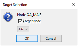
Note that pressing T, while double-clicking a state within a Monitor, also allows setting the Target Node and the Target State.
Augmented Naive Bayes Learning
Now that the Target Node is defined, we have an array of Supervised Learning algorithms available. Given the small number of nodes, variable selection is not an issue and hence this should not influence our choice of algorithm. Furthermore, the number of observations does not create a challenge in terms of computational effort. With these considerations, and without going into further detail, we select the Augmented Naive Bayes algorithm. “Naive” refers to a network structure in which the Target Node is connected directly to all other nodes. Such a Naive Bayes structure is generated by specification, rather than by machine learning. The “augmented” part in the name of this algorithm refers to the additional unsupervised search that is performed on the basis of the given naive structure.
We start the learning process from the menu by selecting Menus > Learning > Supervised Learning > Augmented Naive Bayes. Upon completion of the learning process, we apply the Automatic Layout algorithm P, and BayesiaLab presents the following new network structure.
The predefined Naive Bayes structure is highlighted with the dotted arcs, while the augmented arcs (from the additional Unsupervised Learning) are shown with solid arcs.
Once the network is learned, bringing up the Mapping function and selecting Pearson Correlation for the Arc Analysis provides an instant survey of the dynamics in the network.

As always, the caveat applies that Pearson Correlation should only be interpreted as such if the assumption of linearity can be made.
Structural Coefficient Analysis
Even if we find everything to be reasonable, we will need to ask the question of whether this model does include all important interactions. Did we learn a reliable model that can be generalized? Is the model we built the best one among all the possible networks? Is the model possibly overfitted to the data?
Some of these questions can be studied with BayesiaLab’s Structural Coefficient Analysis. Before we delve into this function, we first need to explain the Structural Coefficient (SC). It is a kind of significance threshold that can be adjusted by the analyst and that influences the degree of complexity of the induced network.
By default, this Structural Coefficient is set to 1, which reliably prevents the learning algorithms from overfitting the model to the data. In studies with relatively few observations, the analyst’s judgment is needed for determining a possible downward adjustment of this parameter. On the other hand, when data sets are large, increasing the parameter to values greater than 1 will help manage the network complexity.
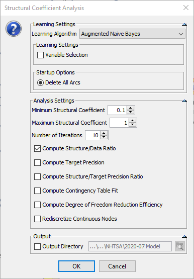
BayesiaLab can systematically examine the question of optimal complexity with the Structural Coefficient Analysis. In our example, we wish to know whether a more complex network, while avoiding overfit, would better capture the dynamics of our domain. Structural Coefficient Analysis generates several metrics that can help in making this trade-off between complexity and fit: Menus > Tools > Multi-Run > Structural Coefficient Analysis.
BayesiaLab prompts us to specify the range of the Structural Coefficient to be examined and the number of iterations to be performed. It is worth noting that the Minimum Structural Coefficient should not be set to 0, or even close to 0. A value of 0 would lead to learning a fully connected network, which can take a long time depending on the number of variables, or even exceed the memory capacity of the computer running BayesiaLab.
The Number of Iterations determines the steps to be taken within the specified range of the Structural Coefficient. We leave this setting at the default level of 10. For metrics, we select Compute Structure/Data Ratio, which we will subsequently plot.
The resulting report shows how the network changes as a function of the Structural Coefficient. For other analyses based on Cross-Validation, this report can be used to determine the degree of confidence we should have in any particular arc in the structure.
Our overall objective here is to determine the correct level of network complexity for representing the interactions with the Target Node without the overfitting of data. By clicking Curve we can plot the Structure/Data Ratio (y-axis) over the Structural Coefficient (x-axis).
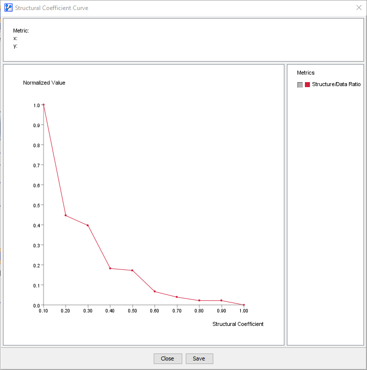
Typically, the “elbow” of the L-shaped curve above identifies a suitable value for the Structural Coefficient (SC). The visual inspection suggests that an SC value of around 0.35 would be a good candidate. Further to the left of this point, e.g. SC≈0.1, the complexity of the model increases much more than the likelihood of the data given the model. This means that arcs would be added without any significant gain in terms of better representing the data. That is the characteristic pattern of overfitting, which is what we want to avoid.
Given the results from this Structural Coefficient Analysis, we can now relearn the network with an SC value of 0.35. The SC value can be set via Graph Panel Contextual Menu > Edit Structural Coefficient or Menus > Edit > Edit Structural Coefficient.

Once we relearn the network, using the same Augmented Naive Bayes algorithm as before, we obtain a more complex network.
Example 2: Seat Belt Usage
Similar to the analysis we performed earlier on Number of Lanes, Speed Limit, and Deformation Location, we will now examine the Target Node, Maximum Known Occupant AIS. We select and double-click the nodes and Manual Belt System Use to bring them up in the Monitor Panel.
Initially, the Monitors show Maximum Known Occupant AIS and Manual Belt System Use with their marginal distributions (1st column from left). We now set evidence on Manual Belt System Use to evaluate the changes to Maximum Known Occupant AIS. Our experience tells us that not wearing a seatbelt is associated with an increased risk of injury in an accident.
Indeed, this is precisely what we observe. For example, for Manual Belt System Use=Not Used the probability of no/minor injury is 66.87% (2nd column). On the other end of the injury spectrum, the probability of serious injuries is 8.21%.
The situation is much better for Manual Belt System Use=Used (3rd column). The probability of no/minor injury is higher (+19.2 percentage points), and the probability of serious injury is much lower (-5.7 percentage points). These results appear intuitive and are in sync with our domain knowledge.
However, does this confirm that wearing a seat belt reduces the risk of sustaining a serious injury by roughly two-thirds? Not yet.
We can further examine this by including the variable . The bottom-left Monitor shows the marginal distribution of Air Bag System Deployed.
To compare the conditions Manual Belt System Use=Not Used and Manual Belt System Use=Used, we first set evidence on Not Used (2nd column, 2nd row). The posterior distribution of Maximum Known Occupant AIS has an expected value of 1.341, and the probability of Air Bag System Deployed=Deployed has increased to 63.71%. Because Maximum Known Occupant AIS has an ordinal rather than numerical scale, we need to be careful when interpreting its expected values (means).
Setting the evidence Manual Belt System Use=Used (3rd column, 2nd row) changes the expected value of Maximum Known Occupant AIS to 0.860, a decrease of 0.481, but it is also associated with a much different posterior distribution of Air Bag System Deployed, which now has a lower probability for Deployed. How should we interpret this?
As it turns out, many airbag systems are designed in such a way that their deployment threshold is adjusted when occupants are not wearing seat belts (Bosch Automotive Handbook, 2011, p. 933). This means that not wearing a seat belt causes the airbag to be triggered differently. So, beyond the direct effect of the seat belt, whether or not it is worn indirectly influences the injury risk via the trigger mechanism of the airbag system.
Covariate Imbalance
Beyond the link between seat belt and airbag, there are numerous other relevant relationships. For instance, seat belt users are more likely to be female, they are older and they are, for some unknown reason, less likely to be involved in a frontal crash, etc.
Similar to the earlier example, the evidence set on Manual Belt System Use is propagated omnidirectionally through the network, and the posterior distributions of all nodes are updated. The Monitors below show the difference between the evidence Manual Belt System Use=Not Used (left set of panels) and Manual Belt System Use=Used (right).
This highlights that seat belt users and non-users are quite different in their characteristics and thus not directly comparable. So, what is the benefit of the seat belt, if any?
In fact, this is a prototypical example of the challenges associated with observational studies. By default, observational studies, like the one here, permit only observational inference. However, performing observational inference on Maximum Known Occupant AIS given Manual Belt System Use is of limited use for the researcher or the policymaker. How can we estimate causal effects with observational data? How can we estimate the (hopefully) positive effect of the seat belt?
Within a traditional statistical framework, a number of approaches would be available to address such differences in characteristics, including stratification, adjustment by regression, and covariate matching (e.g. Propensity Score Matching). For this tutorial, we will proceed with a method that is similar to covariate matching; however, we will do this within the framework of Bayesian networks.
Likelihood Matching with BayesiaLab
We will now briefly introduce the Likelihood Matching (LM) algorithm, which was originally implemented in the BayesiaLab software package for “fixing” probability distributions of an arbitrary set of variables, thus allowing us to easily define complex sets of soft evidence. The Likelihood Matching algorithm searches for a set of likelihood distributions, which, when applied on the Joint Probability Distribution (JPD) encoded by the Bayesian network, allows obtaining the posterior probability distributions defined (as constraints) by the user.
This allows us to perform matching across all covariates while taking into account all their interactions, and thus to estimate the direct effect of Manual Belt System Use. We will now illustrate a manual approach for estimating the effect; in the next chapter, we will show a more automated approach with the Direct Effects function.
Fixing Distributions
We start with the marginal distributions of all nodes. Next, we select all covariate nodes in the Monitor Panel and then select Monitor Contextual Menu > Fix Probabilities.

This “fixes” the (marginal) distributions of these covariate nodes. Their new fixed condition is indicated by the purple color of the bars in the Monitors.
If we now set the evidence on Manual Belt System Use=Used, we will see no significant changes in these fixed covariate distributions. The Likelihood Matching algorithm has indeed obtained materially equivalent distributions.
Causal Inference
Given that the covariate distributions remain fixed, we can now exclusively focus on the Target Node Maximum Known Occupant AIS:
Manual Belt System Use=Not Used
Manual Belt System Use=Used
If we make the assumption that no other unobserved confounders exist in this domain, we will now be able to give the change in the distribution of Maximum Known Occupant AIS a causal interpretation. This would represent the difference between forcing all drivers to wear a seat belt versus forcing all of them not to do so.
More formally we can express such an intervention with Pearl’s do-operator, which reflects actively setting of a condition (or intervention) versus merely observing a condition:
Observational Inference:
In words: the probability of Maximum Known Occupant AIS taking on the value “4-6” given (“|”) that Manual Belt System Use is observed as “Used.”
P(Maximum Known Occupant AIS=4-6|Manual Belt System Use=Not Used)=8.21%
Causal Inference:
In words: the probability of Maximum Known Occupant AIS taking on the value “4-6” given (“|”) that Manual Belt System Use is actively set (by intervention) to “Used.”
P(Maximum Known Occupant AIS=4-6|do(Manual Belt System Use=Used))=2.71%
P(Maximum Known Occupant AIS=4-6|do(Manual Belt System Use=Not Used))=5.99%
From these results we can easily calculate the causal effect:
P(Maximum Known Occupant AIS=4-6|do(Manual Belt System Use=Used)) - P(Maximum Known Occupant AIS=4-6|do(Manual Belt System Use=Not Used)) = -3.28%
We conclude that this difference, -3.28 percentage points, is the “seat belt effect” with regard to the probability of serious injury. Analogously, the effect for moderate injuries is -10.14 percentage points. Finally, for no/minor injuries, there is a positive effect of 13.4 percentage points.
With “causal inference” formally established and implemented through this workflow, we can advance to the principal question of this study, the influence of vehicle size and weight on injury risk.
Effect of Weight and Size on Injury Risk
Our previous example regarding seat belt usage illustrated the challenges of estimating causal effects from observational data. It became clear that the interactions between variables play a crucial role. Furthermore, we have shown how Likelihood Matching, under the assumption of no unobserved covariates, allows us to estimate the causal effect from observational data.
Lack of Covariate Overlap
Before we continue with the effect estimation of vehicle weight and size, we will briefly review the distributions of the nodes under study, Vehicle Curb Weight, and Footprint as a function of Truck Weight Code. We can use this code to select classes of vehicles, including Passenger Car, Truck < 6,000 lbs., and Truck < 10,000 lbs.
We can see that the distributions of Vehicle Curb Weight and Footprint are very different between these vehicles’ classes. For Truck Weight Code=Passenger Car, we have virtually no observations in the two highest bins of Vehicle Curb Weight (left column), whereas for large trucks (Truck Weight Code=Truck < 10,000 lbs.) the two bottom bins are almost empty (right column). We see a similar situation for Footprint.
This poses two problems: Firstly, we now have a rather “coarse” discretization of values within each class of vehicles, which could potentially interfere with estimating the impact of small changes in these variables. Secondly, and perhaps more importantly, the lack of covariate overlap may prevent the Likelihood Matching algorithm from converging on matching likelihoods between variables. As a result, we might not be able to carry out any causal inference. Hence, we must digress for a moment and resolve this issue in the following section on Multi-Quadrant Analysis.
Multi-Quadrant Analysis
BayesiaLab offers a way to conveniently overcome this fairly typical problem. We can perform a Multi-Quadrant Analysis that will automatically generate a Bayesian network for each vehicle subset, i.e. Passenger Car, Truck < 6,000 lbs., and Truck < 10,000 lbs.
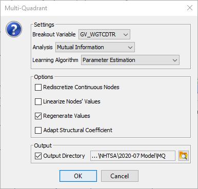
The Multi-Quadrant Analysis can be started via Menus > Analysis > Visual > Segment > Multi-Quadrant.
We now need to set several options: The Breakout Variable (or selector variable) must be set to Truck Weight Code, so we will obtain one network for each state of this node. By checking Regenerate Values, the values of each state of each (continuous) node are re-computed from the data of each subset database, as defined by the Breakout Variable. Rediscretize Continuous Nodes is also an option in this context, but we will defer this step and later perform the re-discretization manually. Finally, we set an output directory where the newly generated networks will be saved.
Upon completion of this step, BayesiaLab presents a set of plots, one for each state of the Breakout Variable, Truck Weight Code.
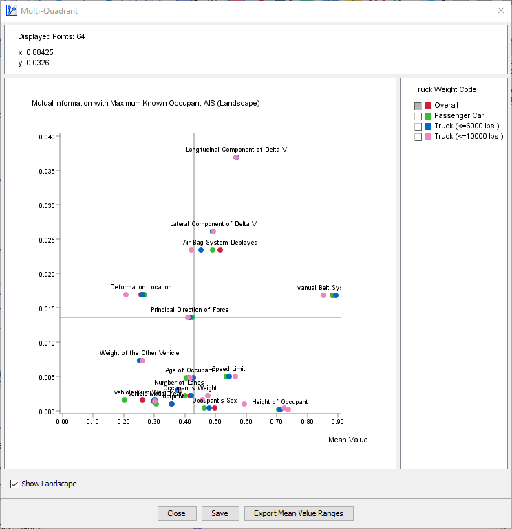
These plots allow us to compare the Mutual Information of each node in the network with regard to the Target Node, Maximum Known Occupant AIS. These plots can be very helpful in determining the importance of individual variables in the context of their respective subset.
In our example, we will omit to go into further detail here and instead inspect the newly generated networks. We can simply open them directly from the previously specified location. The new file names follow this format: original filename & “_MULTI_QUADRANT_” & Breakout Variable State & “.xbl”
Vehicle Class: Passenger Car
When opening the Passenger Car file, we will notice that the structure is exactly the same as in the network that applied to the whole set. However, examining the Monitors will reveal that the computed probabilities now apply to the Passenger Car subset only.
Since Truck Weight Code now only contains a single state at 100%, i.e. the same for each record in the Passenger Car subset, we can go ahead and remove this node from the network. We first select the node and then hit the delete key.
Now we can focus our attention on the two variables that prompted the Multi-Quadrant Analysis, namely Vehicle Curb Weight and Footprint. By double-clicking on Vehicle Curb Weight we bring up the Node Editor, which allows us to review and adjust the discretization of this particular node.
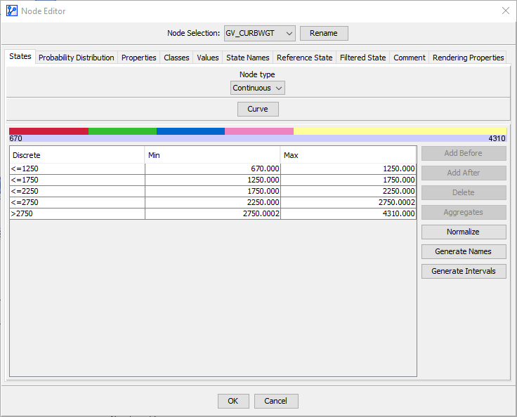
We could directly change the thresholds of the bins in this table. However, it is helpful to bring up the Density Function after clicking on Curve.
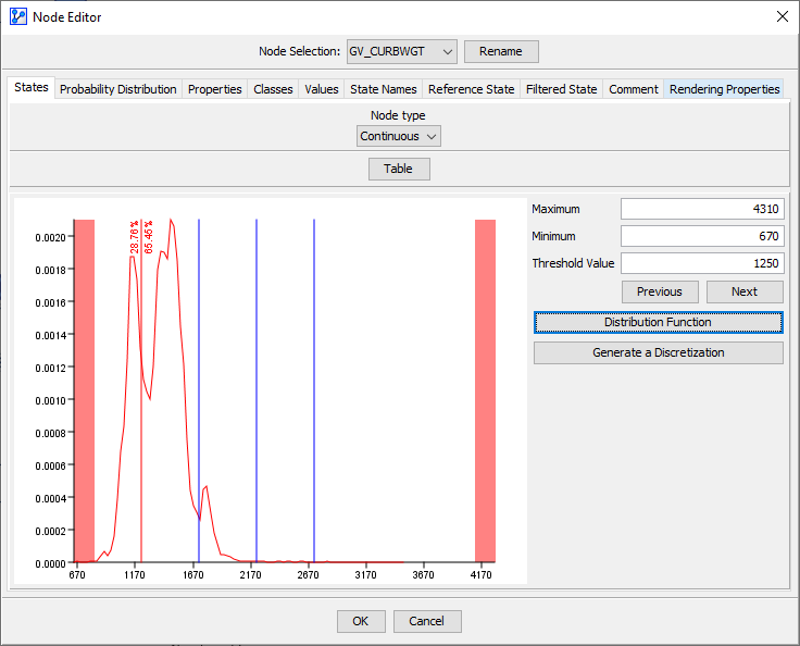
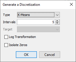
We can now use one of BayesiaLab’s discretization algorithms to establish new bins that are more suitable for the distribution of Vehicle Curb Weight within the Passenger Car subset. Here, we will use the K-Means algorithm with five intervals.
Upon discretization, the new bin intervals are highlighted in an updated PDF plot.
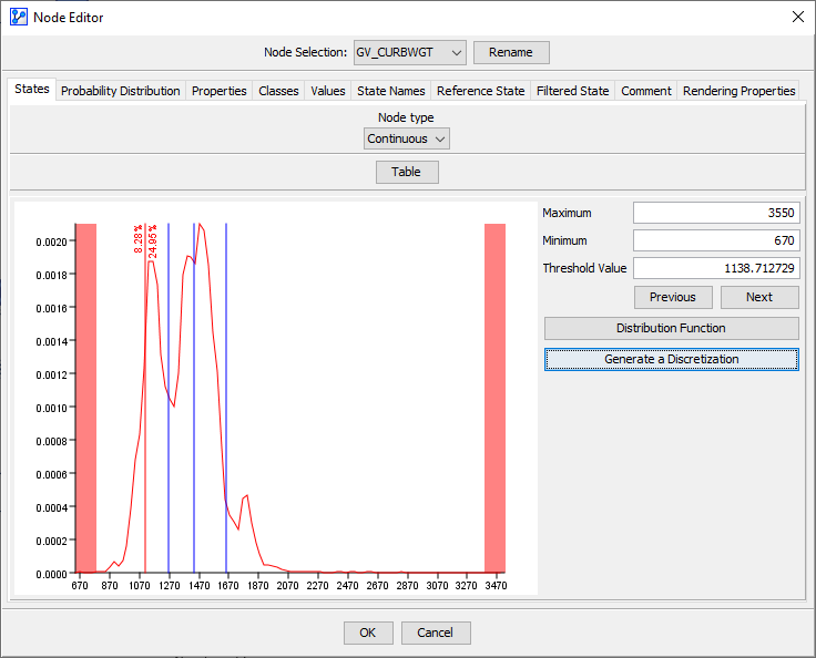
Instead of automatically determining the bins, we could also manually specify them. In our case, we take the bins proposed by the K-Means algorithm and round them to the nearest 50 kg:
We apply the same approach for Footprint and present the result in the following Monitor.
Both discretizations now adequately capture the underlying distributions of the respective variables within the subset Passenger Car.
We now proceed to our principal question of how Vehicle Curb Weight and Footprint affect Maximum Known Occupant AIS. It might be tempting to immediately apply the same process as with the seat belt effect estimation, i.e. fix all covariates with Likelihood Matching and then simulate the response of Maximum Known Occupant AIS as a function of changing values of Vehicle Curb Weight and Footprint. Indeed, we wish to keep everything else the same in order to determine the exclusive Direct Effects of Vehicle Curb Weight and Footprint on Maximum Known Occupant AIS.
However, fixing must not apply to all nodes. Following the definition of kinetic energy,
Energy Absorption is a function of Vehicle Curb Weight, Longitudinal Component of Delta V, and Lateral Component of Delta V.
This means that Energy Absorption cannot be maintained at a fixed distribution as we test varying values of Vehicle Curb Weight and Footprint.
It is important to understand that the relationship of Vehicle Curb Weight versus Energy Absorption is different from, for instance, Vehicle Curb Weight versus Longitudinal Component of Delta V or Lateral Component of Delta V. The node must be allowed to “respond” in our simulation, as in observational inference, while Longitudinal Component of Delta V or Lateral Component of Delta V have to be kept at a fixed distribution.
Non-Confounders
BayesiaLab offers a convenient way to address this requirement. We can assign a special pre-defined Class to variables like Energy Absorption, called Non_Confounder. We can assign a Class by right-clicking the node and selecting Properties > Classes > Add from the Contextual Menu.
Now, we select the Predefined Class Non_Confounder from the drop-down menu.

The Class icon in the bottom right corner of the screen indicates that a Class has been set.
Direct Effects
The principal question of this study now adds one further challenge in that we are looking for the effect of a continuous variable, Vehicle Curb Weight, as opposed to the effect of a binary variable, such as Manual Belt System Use. This means that our Likelihood Matching algorithm must now find matching confounder distributions for a range of values of Vehicle Curb Weight and Footprint.
As opposed to manually fixing distributions via the Monitors, we now use BayesiaLab’s Direct Effects function that performs this automatically. Thus, all Confounder nodes will be fixed in their distributions, excluding the nodes currently being manipulated, the Target Node, and the Non-Confounder nodes.
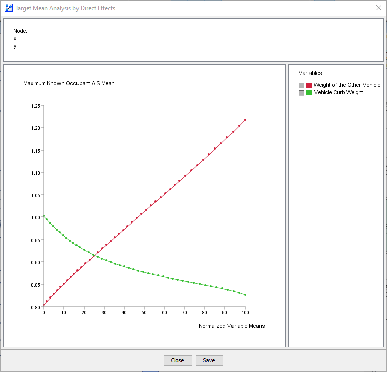
Although we are primarily interested in the effect of Vehicle Curb Weight and Footprint on Maximum Known Occupant AIS, we will also consider another weight-related node, i.e. Weight of the Other Vehicle, which represents the curb weight of the other vehicle involved in the collision. Given the principle of conservation of linear momentum, we would expect that, everything else being equal, increasing the weight of one’s own vehicle would decrease injury risk, while an increase in the weight of the collision partner would increase injury risk.
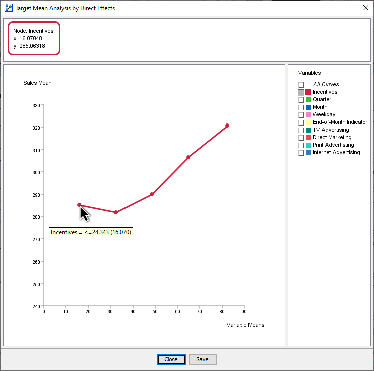
We can select these three nodes in the network and then perform a Target Mean Analysis by Direct Effect by selecting Analysis > Visual > Target > Target's Posterior > Curves > Direct Effects.
Given that only a subset of nodes was selected, we are prompted to confirm this set of three nodes.
In our case, we have different types of variables, e.g. Footprint, measured in m2, and Vehicle Curb Weight and Weight of the Other Vehicle, measured in kg. As such, they could not be properly presented in a single plot, unless their x-ranges were normalized. Thus, it is helpful to select Normalize from the options window.
Once this is selected, we can continue to Display Sensitivity Chart.

The Direct Effects curves of Vehicle Curb Weight and Weight of the Other Vehicle have the expected slope. However, Footprint appears “flat,” which is somewhat counterintuitive.
Alternatively, we can exclusively focus on Vehicle Curb Weight and Weight of the Other Vehicle, which allows us to look at them on their original scales in kilograms. Thus, we select Mean instead of Normalize as the display option.
Note that the Vehicle Curb Weight range is smaller than that of Weight of the Other Vehicle, which was not apparent on the normalized scale. With the Multi-Quadrant Analysis, we had previously generated specific networks for each vehicle class. As a result, the range of Vehicle Curb Weight in each network’s database is delimited by the maximum and minimum values of each vehicle class. Furthermore, the maximum and minimum values that can be simulated within each network are constrained by the highest and lowest values that the states of the node can represent. We can easily see these limits in the Monitors.

For Passenger Car, Vehicle Curb Weight ∈ [1133.912, 1807.521]. This also means that we cannot simulate outside this interval and are thus unable to make a statement about the shape of the Direct Effects curves outside these boundaries.
However, within this interval, the simulated Direct Effects curves confirm our a priori beliefs based on the laws of physics regarding the effects of vehicle mass. As both curves appear fairly linear, it is reasonable to have BayesiaLab estimate the slope of the curves around their mean values. We do this by selecting Menus > Analysis > Report > Target > Direct Effects on Target.
A results window shows the estimated Direct Effects in table format.
These Direct Effects can be interpreted similarly to coefficients in a regression. This means that increasing Vehicle Curb Weight by 100 kg would bring about a 0.02 decrease in the expected value of Maximum Known Occupant AIS. On a 0-6 scale, this may seem like a minute change.
However, a negligible change in the expected value (or mean) can “hide” a substantial change in the distribution of Maximum Known Occupant AIS, which is illustrated below. An increase of 0.02 in the expected value translates into an 8% (or 0.3 percentage points) increase in the probability of a serious or fatal injury.
In the example, the changes in the probability of serious injury are in the order of magnitude of one-tenth of one percent. These numbers may appear minute, but they become fairly substantial when considering that roughly 10 million motor vehicle accidents occur in the United States every year. For instance, an increase of 0.1 percentage points in the probability of serious injury would translate into 10,000 human lives that are profoundly affected.
Entire Vehicle Fleet
At the beginning of this section on effect estimation, we made a case for Multi-Quadrant Analysis due to a lack of complete covariate overlap. Consequently, we could only estimate the effects of size and weight by vehicle class. However, the big picture remains of interest. What do these effects look like across all vehicle classes? Despite our initial concerns regarding the lack of overlap, would it perhaps be possible to “zoom-out” to assess these dynamics for the entire vehicle fleet? We will now attempt to do just that and perform inference at the fleet level. There is, unfortunately, no hard-and-fast rule that tells us in advance what amount of overlap is sufficient to perform inference correctly. However, BayesiaLab contains a built-in safeguard and alerts us when Likelihood Matching is not possible.
Keeping the above caveats in mind, we return to our original network, i.e. the one we had learned before applying the Multi-Quadrant Analysis. We now wish to see whether the class-specific effects are consistent with fleet-level effects.
Our fleet-level model turns out to be adequate after all, and the Likelihood Matching algorithm does return results that appear similar to the results for the analysis of the Passenger Car model.
Simulating Interventions
Thus far, we have only computed the impact of reducing Vehicle Curb Weight while leaving the distribution of Weight of the Other Vehicle the same. This means we are simulating as to what would happen if a new fleet of a lighter fleet of vehicles were introduced, facing the older, heavier fleet. This simplification may be reasonable as long as the new fleet is relatively small compared to the existing one. However, in the long run, the distribution of Weight of the Other Vehicle would inevitably have to become very similar to GV_CURBWGT.
In order to simulate such a long-run condition, any change in the distribution of Vehicle Curb Weight would have to be identically applied to Weight of the Other Vehicle. This means once we set evidence on Vehicle Curb Weight (and fixed its distribution) we need to set the same distribution on Weight of the Other Vehicle (and fix it).
Note that we are now performing causal inference, i.e. “given that we do” versus “given that we observe.” Instead of observing the injury risk of lighter vehicles (and all the attributes and characteristics that go along with such vehicles), we do make them lighter (or rather force them by mandate), while keeping all the attributes and characteristics of drivers and accidents the same.
For instance, reducing the average weight of all vehicles to 1,500 kg appears beneficial. The risk of serious or fatal injury drops to 2.85%. Considering these simulated results, this may appear as a highly desirable scenario. This would theoretically support a policy that “lightens” the overall vehicle fleet by government mandate. However, we must recognize that such a scenario may not be feasible as functional requirements of vans and trucks could probably not be met within mandatory weight restrictions.
Alternatively, we could speculate about a scenario in which there is a bimodal distribution of vehicle masses. Perhaps all new passenger cars would become lighter (again by government mandate), whereas light trucks would maintain their current weights due to functional requirements. Such a bimodal scenario could also emerge in the form of a “new and light” fleet versus an “old and heavy” existing fleet. We choose a rather extreme bimodal distribution to simulate such a scenario, consciously exaggerating to make our point.
As opposed to a homogeneous scenario of having predominantly light vehicles on the road, this bimodal distribution of vehicles increases the injury risk versus the baseline. This suggests that a universally lighter fleet, once established, would lower injury risk, while a weight-wise diverse fleet would increase risk.
These simulations of various interventions highlight the challenges that policymakers face. For instance, would it be acceptable, with the objective of long-term societal safety benefit, to mandate the purchase of lighter vehicles, if this potentially exposed individuals to increased injury risk in the short term? What are the ethical considerations with regard to trading off “probably more risk now for some” versus “perhaps less risk later for many”? It appears difficult to envision a regulatory scenario that will benefit society as a whole, without any adverse effects to some subpopulation, at least for some period of time. However, it clearly goes beyond the scope of our paper to elaborate on the ethical aspects of weighing such risks and benefits.
Summary
- This paper was developed as a case study for exhibiting the analytics and reasoning capabilities of the Bayesian network framework and the BayesiaLab software platform.
- Our study examined a subset of accidents with the objective of understanding injury drivers at a detail level, which could not be fully explored with the data and techniques used in the context of the EPA/NHTSA Final Rule.
- For an in-depth understanding of the dynamics of this problem domain, it was of great importance to capture the multitude of high-dimensional interactions between variables. We achieved this by learning Bayesian networks with BayesiaLab.
- On the basis of the Bayesian networks learned from data, BayesiaLab’s Likelihood Matching was used to estimate the exclusive Direct Effects of individual variables on the outcome variable. The estimated effects were generally consistent with prior domain knowledge and the laws of physics.
- Simulating domain interventions, e.g. the impact of regulatory action required carrying out causal inference, using Likelihood Matching. We emphasized the distinction between observational and causal inference in this context.
- With regard to this particular collision type, we conclude that injury risk remains a function of both mass and size. More specifically, as a result of decomposing the individual effects of vehicle size and weight, the notion of “mass reduction being safety-neutral given a fixed footprint” could not be supported in this specific context at this time.
Conclusion
Learning Bayesian networks from historical accident data using the BayesiaLab software platform allows us to comprehensively and compactly capture the complex dynamics of real-world vehicle crashes. With the domain encoded as a Bayesian network, we can “embrace” the high-dimensional interactions and leverage them for performing observational and causal inference. By employing Bayesian networks, we provide an improved framework for reasoning about vehicle size, weight, injury risk, and ultimately about the consequences of regulatory intervention.
References
2017 and Later Model Year Light-Duty Vehicle Greenhouse Gas Emissions and Corporate Average Fuel Economy Standards. Final Rule. Washington, D.C.: Department of Transportation, Environmental Protection Agency, National Highway Traffic Safety Administration, October 15, 2012. https://federalregister.gov/a/2012-21972 .
2017 and Later Model Year Light-Duty Vehicle Greenhouse Gas Emissions and Corporate Average Fuel Economy Standards. Department of Transportation, Environmental Protection Agency, National Highway Traffic Safety Administration, August 28, 2012.
A Dismissal of Safety, Choice, and Cost: The Obama Administration’s New Auto Regulations. Staff Report. Washington, D.C.: U.S. House of Representatives Committee on Oversight and Government Reform, August 10, 2012.
Bastani, Parisa, John B. Heywood, and Chris Hope. U.S. CAFE Standards - Potential for Meeting Light-duty Vehicle Fuel Economy Targets, 2016-2025. MIT Energy Initiative Report. Massachusetts Institute of Technology, January 2012.

Chen, T. Donna, and Kara M. Kockelman. “THE ROLES OF VEHICLE FOOTPRINT, HEIGHT, AND WEIGHT IN CRASH OUTCOMES: APPLICATION OF A HETEROSCEDASTIC ORDERED PRO-BIT MODEL.” In Transportation Research Board 91st Annual Meeting, 2012. http://www.ce.utexas.edu/prof/kockelman/public_html/TRB12CrashFootprint.pdf .
“Compliance Question - Will Automakers Build Bigger Trucks to Get Around New CAFE Regulations?” Autoweek. Accessed September 9, 2012. http://www.autoweek.com/article/20060407/free/60403023.
Conrady, Stefan, and Lionel Jouffe. “Causal Inference and Direct Effects - Pearl’s Graph Surgery and Jouffe’s Likelihood Matching Illustrated with Simpson’s Paradox and a Marketing Mix Model,” September 15, 2011.
Conrady, Stefan, and Lionel Jouffe. Case Study: Modeling Vehicle Choice and Simulating Market Share
“Crashworthiness Data System - 2009 Coding and Editing Manual.” U.S. Department of Transportation National Highway Traffic Safety Administration, January 2009.
“Crashworthiness Data System - 2010 Coding and Editing Manual,” n.d.