
Optimization and Recommendations
Variations within the Realm of the Possible
This view is interesting on its own; however, we can more formally utilize this information. The position of each model on the attributes’ ranges allows us to compute the “gap to best/extreme level.” This will subsequently become very important as we look for ways to improve brand loyalty.
For instance, with regard to Factor 17, Fit Of Other Body Panels, the Dodge Ram achieves the highest rating, making it an appropriate target for competitors. If we were attempting to improve the rating of the GMC Sierra, the level of the Dodge Ram could be used as a target level.
Because this performance level has already been achieved, it is feasible and therefore realistic. This type of reference is precisely what we require for subsequent optimization. Without such a reference point, an optimization algorithm would happily recommend increasing the rating to a perfect 10, which is not helpful for practical purposes.
BayesiaLab can automatically extract the delta to highest and lowest levels for each factor. In this specific context, we call these deltas Variations. We will utilize these Variations as constraints for the optimization algorithm.
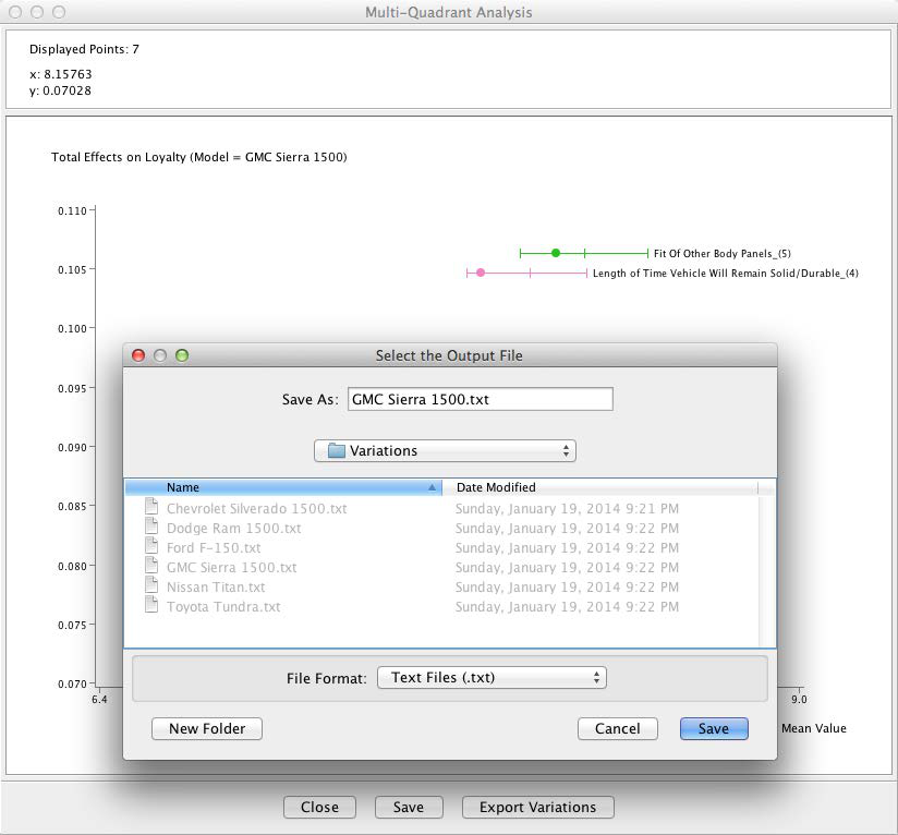
By clicking the Export Variations button, BayesiaLab saves the Variations for the currently selected model. For each model that we wish to optimize, we simply save this data as a text file.
Optimization
The Multi-Quadrant Analysis has generated new networks for each model, plus we have saved the associated Variations. Thus, we have all the components necessary for optimization. For the purpose of this tutorial, we will attempt to optimize the loyalty for the GMC Sierra.
To do so, we open the GMC Sierra-specific file generated by the most recent Multi-Quadrant Analysis.

Before proceeding to the optimization, we will briefly examine the Target Response Functions for the GMC Sierra, which we obtain via Target Mean Analysis (Standard).
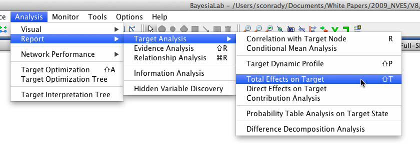
As earlier, when we did this at the segment level, we also ran the Total Effects on Target report: Analysis > Report > Target Analysis > Total Effects on Target.
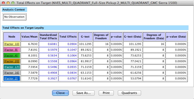
We obtain a report that shows the mean values of each factor, plus the corresponding Total Effects.
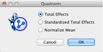
Here, the Quadrant Plot becomes very helpful as it shows both Value and Total Effects in a single plot.
There are many ways to interpret the above plot qualitatively. For instance, we may be tempted to look at Fit of Other Body Panels as the top driver and suggest focusing our efforts there. Also, we might say that Technical Innovations is fairly important, but has room for substantial improvement.
The challenge is to determine which combination of initiatives will yield the maximum improvement for loyalty, and what the new loyalty level would be.
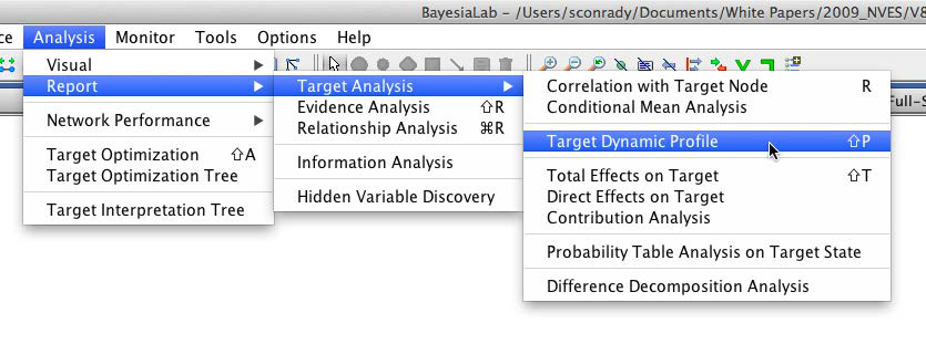
This brings us back to the central purpose of this study. We start optimization by selecting Analysis > Report > Target Analysis > Target Dynamic Profile.
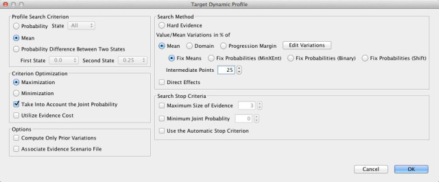
In the following window, we need to select several options that are critical in our search for optimal values. First, we are looking to maximize the mean of Loyalty (rather than, for instance, maximizing the probability of certain repurchase outcomes).
The checkbox Take Into Account Joint Probability is very important in our context. As we optimize, we need to bear in mind that loyalty is expressed as a probability. We might be tempted to look for a scenario in which we obtain 100% loyalty. However, the absolute number of units sold as a result of loyalty is critical from a business perspective. For instance, 100% loyalty within a niche of 100 customers generates fewer sales (i.e., 100 units) than an average loyalty of 50% among a larger group of 1,000 customers (i.e., 500 units).
So, pursuing an idealized state of perfect loyalty may be counterproductive as it might narrow the available customer base. This is where Joint Probability becomes an extremely helpful concept. By virtue of having learned a Bayesian network, we automatically have the joint probability of every conceivable combination of values of all nodes. This provides us with the ability to assess how far our optimized scenarios depart from the current reality. Considering this “stretch” beyond the status quo is central to our optimization approach.
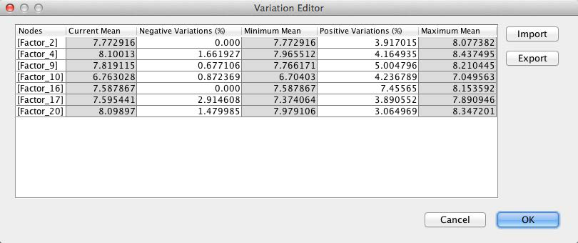
The second “reality check” relates to the variations, which we discussed earlier. By default, the Variation Editor is set to ±100%. This is what we see when we first open it.
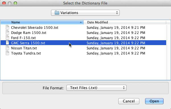
Now we re-introduce the variations we obtained earlier. By clicking Import, we can select the previously saved file with the Variations for the GMC Sierra.
With the Variations loaded, we see the ranges within which the optimization value can search for the optimal combination of values.
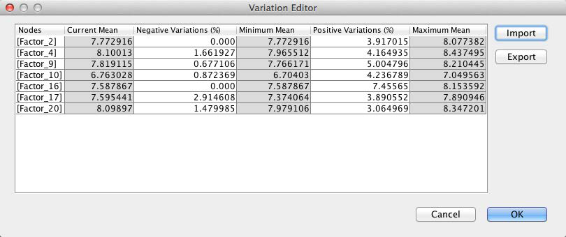
Clicking OK immediately starts the optimization routine. Given the small size of the network, the optimization report pops up within seconds.
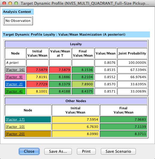
For a more detailed explanation, we save this report as an HTML file, which we can then open in Excel for further annotation. This file keeps all the formatting, including color-coding, of the on-screen report.
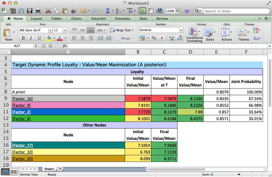
Recommendation for GMC Sierra 1500
The above report presents the results in a highly-condensed format. It will be helpful to dissect this table cell by cell. To properly interpret this table, it should be read line by line, top to bottom.
This table clearly spells out the top priorities for the GMC Sierra 1500. According to this simulation, achieving the new levels of the factors would lift loyalty from 0.80 to 0.85. For the GMC, this would translate into several thousand more customers returning to the brand.
For reference, the factor-to-manifest mapping is provided in the appendix below.
Given that the earlier Multi-Quadrant Analysis generated networks for all models in this segment, we could now repeat the optimization for any of the other models within minutes.