Latent Factor Induction

Latent Factor Induction via Multiple Clustering

As our next step, we introduce these newly-identified latent factors into our existing network and estimate their probabilistic relationships with the manifest variables. This means we create a new node for each latent factor, adding 24 new dimensions in our network. For this step, we need to return to the Modeling Mode because introducing factor nodes into the network requires learning algorithms.

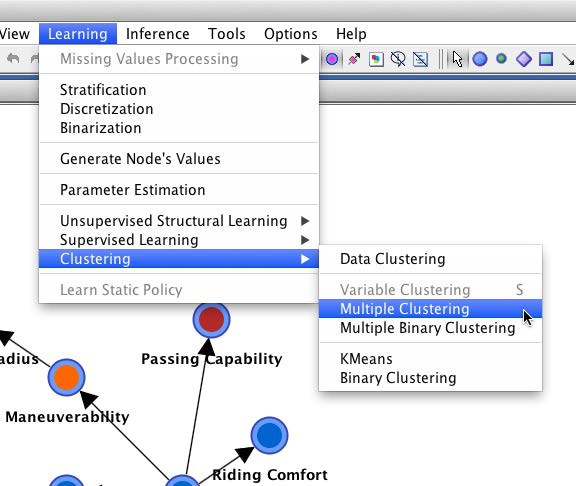
More specifically, we select Learning > Clustering > Multiple Clustering, which brings up the Multiple Clustering dialog.

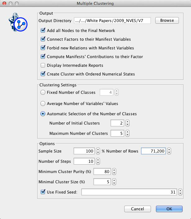
There is a range of settings, but we will focus only on a subset of the available options. First, we need to specify an output directory for the learned subnetworks. Second, we need to set parameters for the clustering process, such as the minimum and maximum number of states that can be created during learning. For our example, we select Automatic Selection of the Number of Classes, which allows the learning algorithm to find the optimum number of factor states up to a maximum of five states. This means that each new factor will need to represent the corresponding manifest variables with up to five states [9].

[9] A complete list of factors and their associated nodes is provided in the appendix.

Upon completion of the Multiple Clustering process, we obtain a new network file that contains one small network for each cluster, with one factor being at the center of each cluster.

The arcs between the factors and their manifest nodes are labeled with Direct Effect Contribution values. This allows us to easily identify the importance of the manifests with regard to their respective factors.

Traditionally, we would now choose a name for each factor so we can interpret factors without looking at their manifests. For instance, $\mathit{Factor\_12}$, shown below, could be called $\mathit{Interior\ Quality}$ or something similar. In BayesiaLab, we can defer this naming process by using the strongest node (based on Direct Effect Contribution) within each cluster as that factor’s Node Comment.

Clicking Display Node Comments in the menu bar will reveal Interior_Trim & Finish_(4) as a label on the factor. The suffix (4) indicates that 4 manifest variables are linked to this factor.

Factor States/Values

Beyond adding the factors to the network, the Multiple Clustering process has also generated states for all factors and computed their values. Inducing a factor means finding an appropriate summary of the underlying joint probability distribution defined by the manifest nodes. In the previous example of $\mathit{Factor\_12}$, this would mean that the states of $\mathit{Factor\_12}$ can summarize the following four nodes: Interior Trim & Finish, Quality of Interior Materials, Interior Colors, and Quality of Seat Materials.

We can examine the factor states and values by opening the network for $\mathit{Factor\_12}$, switching into Validation Mode, and selecting all nodes for display in the Monitor Panel. By default, we see the marginal distributions of all the manifests and the factor.

By sequentially setting evidence on each of the four states of $\mathit{Factor\_12}$, we see what states of the manifests correspond to the factor states.

Looking at these Monitors also provides some intuition regarding the values of the states of $\mathit{Factor\_12}$. BayesiaLab computes these values as the weighted average of the associated manifests’ values. As such, $\mathit{Factor\_12}$ becomes a compact summary of the connected manifest nodes.

Introducing the Target Node

Now that factors have been formally introduced into the network, each representing a major concept, we can proceed to the next step. We will introduce the principal variable of interest in this study, Loyalty, as the target variable.

This node was excluded earlier in the clustering process, so it would not become clustered into a factor. So, the next step is to un-exclude this node, which we do by right-clicking the node and then selecting Properties > Exclusion (shortcut: press X and double-click on the node).

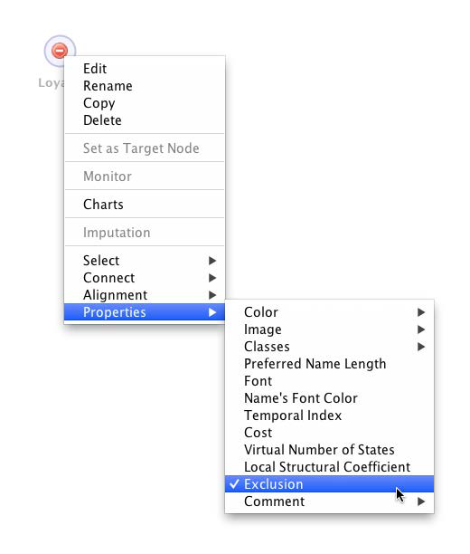
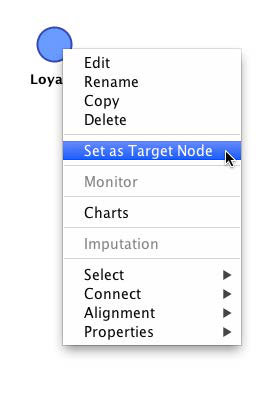
Also, we need to make this node the Target Node. We do this by picking Set as Target Node from the contextual menu. Note that the un-exclusion and the Target Node definition can be done at the same time by pressing T and double-clicking on the excluded node.

Upon introduction of the Target Node, we can interpret the status quo as the first two layers of a hierarchical model, as illustrated below. The outer ring contains the manifest nodes, the inner ring consists of the factors. In the middle, we have the yet-to-be-connected Target Node.

Focusing on Factors

We could continue our analysis with this network as is, including both factors and manifest nodes. However, for practical planning purposes, working with factors, i.e., the major concepts, is typically more relevant. Also, removing the manifest variables will improve the expository clarity of this tutorial. Thus, we will conduct all subsequent analyses exclusively with the factors, rather than the manifest nodes.

To delete the manifest nodes, we right-click on any one of them and then choose Select > Classes.

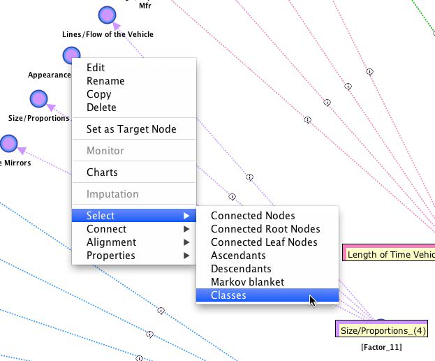
From the pop-up window, we pick Manifest.

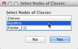
This highlights all manifest nodes, i.e., the outer ring. We can now delete them, either via the Delete key or from the main menu via Edit > Delete Selection.

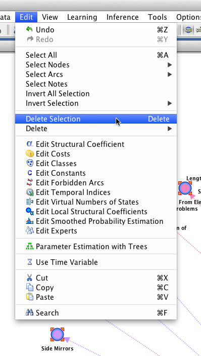
This leaves us with the factors, the Target Node Loyalty, plus the previously excluded nodes, Segment, Make, and Model.