
Unsupervised Learning and Variable Clustering
Unsupervised Structural Learning
A central element in our study is to look for overarching concepts among the 98 satisfaction measures in our dataset. Once identified, these concepts will subsequently serve as factors as we further develop our model.
Machine learning a Bayesian network is a remarkably practical way to identify easily-interpretable variable clusters for factor induction. Among BayesiaLab’s Unsupervised Learning algorithms, the Maximum Weight Spanning Tree is a very efficient approach for quickly obtaining a Bayesian network that can provide the basis for variable clustering. The speed of this particular method is due to a key constraint, namely that in the network to be learned, each node is restricted to having only one parent node. This massively reduces the number of candidate networks that the learning algorithm must examine.
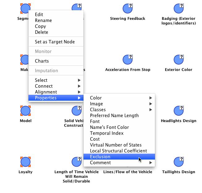
Prior to initiating clustering, we exclude any nodes that should not be part of the clustering process, such as the node we later use as the target node and nodes we use as breakout variables (e.g., Segment). We can exclude nodes by right-clicking selected nodes and choosing Properties > Exclusion from the contextual menu. Alternatively, hold X while double-clicking nodes. Once excluded, nodes appear in the excluded style shown below.
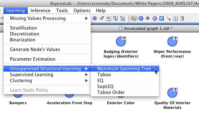
Now we can start the learning process from the main menu: Learning > Unsupervised Structural Learning > Maximum Spanning Tree.
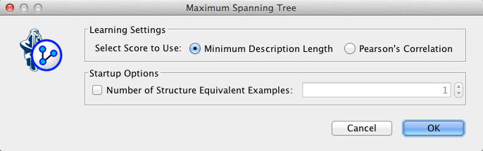
The Maximum Weight Spanning Tree is the only learning algorithm in BayesiaLab that offers an alternative to the Minimum Description Length (MDL) as the learning score. However, without further explanation, we will stick to the default and confirm MDL.
This default view of the resulting network is hardly intuitive. Hence, throughout this exercise, we will make frequent use of one of several available layout algorithms.
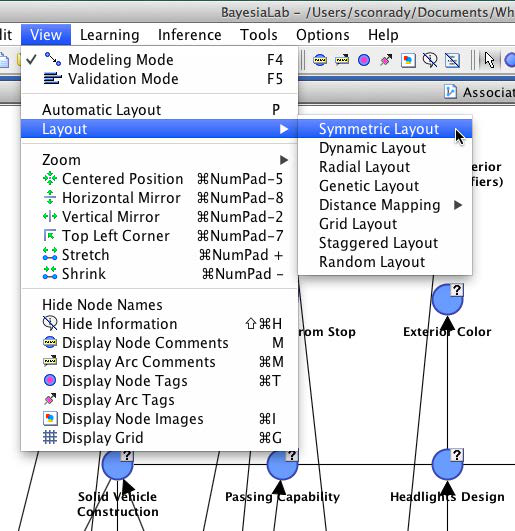
All layout algorithms are accessible from the main menu via View > Layout. Most often, we will use View > Automatic Layout, or alternatively use the shortcut P.
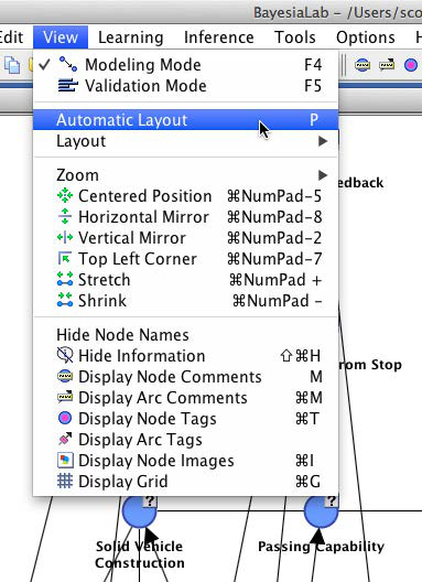
Upon applying a layout algorithm, we obtain an untangled version of the original network. Note that the structure of the network remains unchanged. We can further adjust the positions of the nodes as needed to create a legible and interpretable layout.
In this network, we can examine the probabilistic relationships between the nodes, which are represented as arcs. The structure of the network lends itself to a “sanity check” against our own domain knowledge. For instance, we can look at the lower right branch of the network and see that all these nodes relate to the vehicle interior and seating. It should not surprise us to see that Front Seat Roominess is directly connected to Ease of Front Seat Entry.
Mapping
Beyond this kind of qualitative assessment, BayesiaLab’s Mapping function is very helpful for interpreting the importance of the nodes and the strength of the relationships between them.
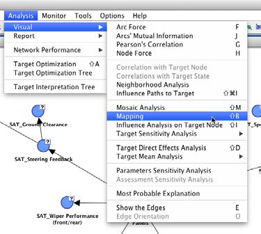
We can initiate Mapping from within the Validation Mode by selecting Analysis > Visual > Mapping.
The Mapping window features drop-down menus for Node Analysis and Arc Analysis. We select Node Force for Node Analysis; for Arc Analysis, we choose Mutual Information.
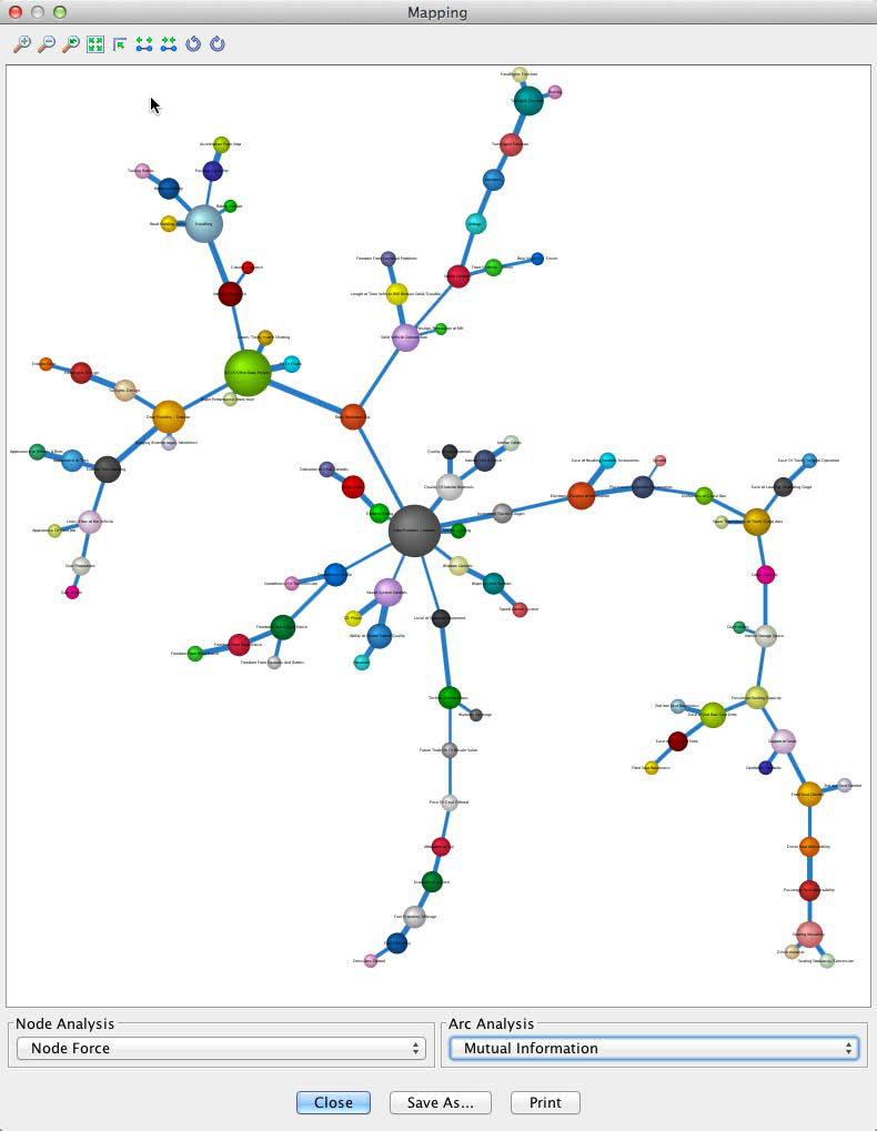
In the resulting graph, as selected, node size reflects the Node Force and arc thickness reflects the Mutual Information. This visualization suggests that Solid Vehicle Construction and Handling are among the most important nodes. All measures appear plausible, so we feel comfortable moving forward on this basis.
Missing Values Imputation
As we already saw during the data import process, all rating variables contain missing values. Given that we set Structural EM as the missing values imputation algorithm, we could proceed with our entire analysis without further thinking about the missing values. The Structural EM algorithm would handle them automatically as we go along [8]. However, there is a significant computational burden associated with this ongoing computation.
To accelerate all subsequent tasks, we will fix the most recent imputation that was generated during the learning of the Maximum Weight Spanning Tree.
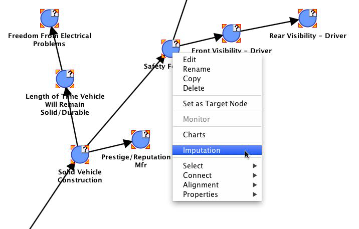
To perform this imputation, we first select all nodes, then right-click on any one of the nodes with missing values, and finally select Imputation from the contextual menu.
We are given a choice of modes, of which we select Standard and Choose the States According to the Law.
Upon completion of the process, all question marks disappear from the network, indicating that there are no more missing values.
[8] For more details, please see our white paper on missing values processing with Bayesian networks: http://bayesia.us/missing-values-processing-with-bayesian-networks.html
Variable Clustering
The network, as we see it here, is intended only as an interim step. For product planning or decision-making purposes, it would indeed be difficult to work directly with 98 manifest nodes. We would not be able to see the proverbial forest for all the trees. Rather, this network will serve as the basis for Variable Clustering, i.e., grouping nodes into meaningful concepts.
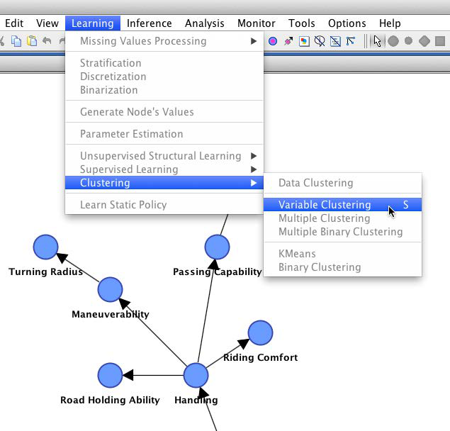
We start this clustering process, from within the Validation Mode, by selecting Learning > Clustering > Variable Clustering (or by using the keyboard shortcut S).
We now see the same graph as before; however, the nodes are now colored according to their proposed cluster membership. In our case, BayesiaLab suggests 26 clusters, as indicated in the menu bar.
We can move the slider to change the number of clusters (or by clicking the arrow buttons). This allows us to align the number of clusters with our domain knowledge. As we change the number, the node colors are automatically updated.
Additionally, we can view a dendrogram while adjusting the number of clusters. Two dendrogram examples are shown below: one with 27 clusters (left) and one with 10 clusters (right).
Alternatively, we can show the currently selected clustering in a format similar to the Mapping function via the menu bar.
For an easier interpretation of these “bubbles”, we can attach labels to them. Since each bubble represents a cluster of nodes, we select Display Best Node Name from the contextual menu.
This shows the name of the node that most strongly contributes to each cluster, given the currently selected number of clusters.
Two screenshots are shown as examples, based on 24 and 10 clusters respectively.
With Dendrogram and Mapping, we can visually experiment until the appropriate cluster number is established. The final selection of the number of clusters remains the task of the analyst. There is no hard-and-fast rule for choosing the number of clusters as this example illustrates. For instance, is it appropriate to cluster nodes related to noise with nodes related to smoothness? Two alternative Dendrograms are shown below. Only a domain expert can make a judgment in this regard.
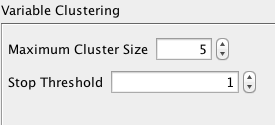
The number of clusters automatically proposed by BayesiaLab is based on two heuristics: the first is based on the strength of the relationships, the second on the maximum number of variables per cluster. Whereas we generally do not advise changing the former, the latter can be modified via Options > Settings > Learning > Variable Clustering.
After further review of all diagrams, we conclude that 24 clusters are most appropriate for this domain and confirm this choice by clicking the Validate Clustering button.
Furthermore, we confirm that we want to keep the colors from the just-completed interactive clustering.
This confirmation generates the Variable Clustering Report, which summarizes each node’s cluster membership.
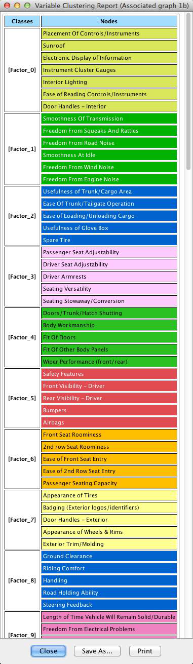
Initially, the clusters are simply labeled as , , …, [9].