Segment and Model-Level Analysis
Multi-Quadrant Analysis (Total Market ➔ Segment)
To study this domain at the level of vehicle segments, we could now start all over again and generate a new network for each segment from scratch. BayesiaLab provides a convenient shortcut for the researcher by means of Multi-Quadrant Analysis.

BayesiaLab can automatically replicate the original model (learned for the entire market) for each state of a specified Breakout Node. This is where the previously excluded node, Segment, comes into play. To make use of it here, we need to un-exclude it at this time.
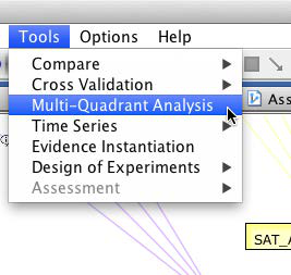
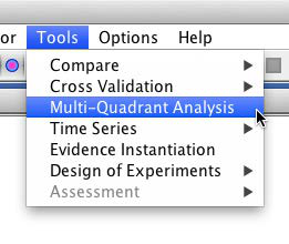
We start the Multi-Quadrant Analysis from the main menu, within Validation Mode, via Tools > Multi-Quadrant Analysis.
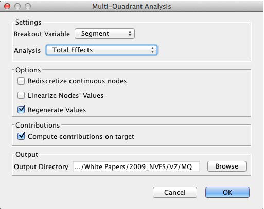
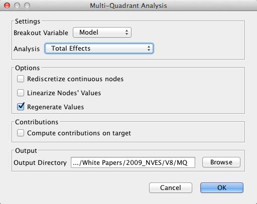
In the following dialog box, we specify the options of the Multi-Quadrant Analysis. Most importantly, we need to select the Breakout Variable, which in our case needs to be Segment. Furthermore, we define an output directory. This is where the segment-level networks will be saved.
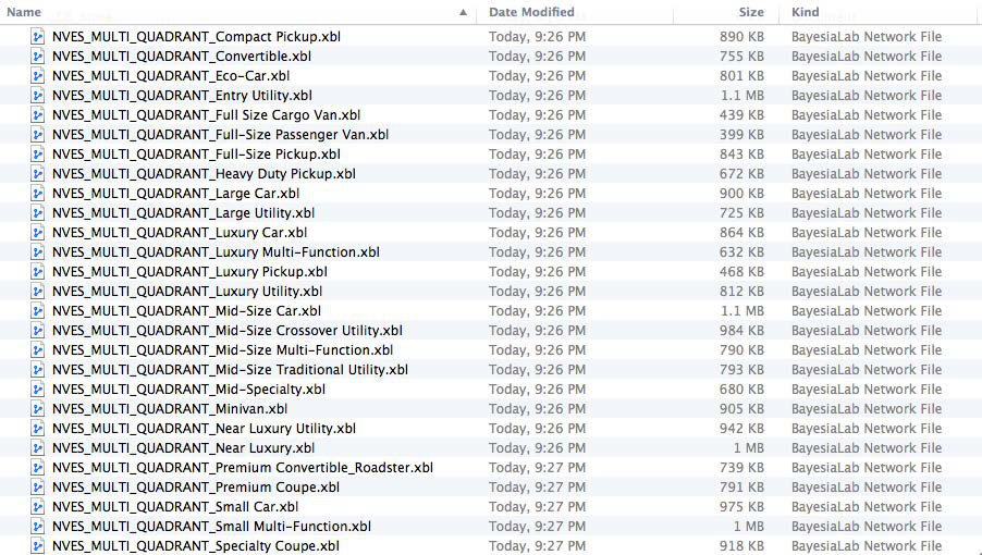
Once this process is completed, all new networks can be found in the specified directory. The file names are created according to the following syntax: Original Network File Name + MULTI_QUADRANT + Breakout Variable State.
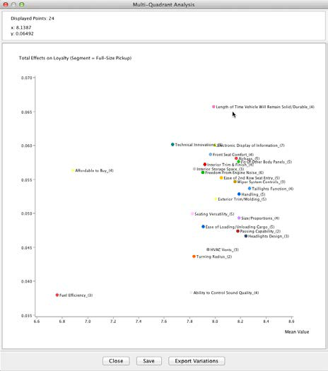
In BayesiaLab itself, we obtain a Quadrant Plot, which shows the Mean Value of each node on the x-axis and the Total Effect on the y-axis (even though quadrants are not explicitly shown here, we will soon explain how a quadrant view can be helpful for interpretation).
This plot exists for all the states of the Breakout Variable, i.e., for all segments. The currently selected state is highlighted.
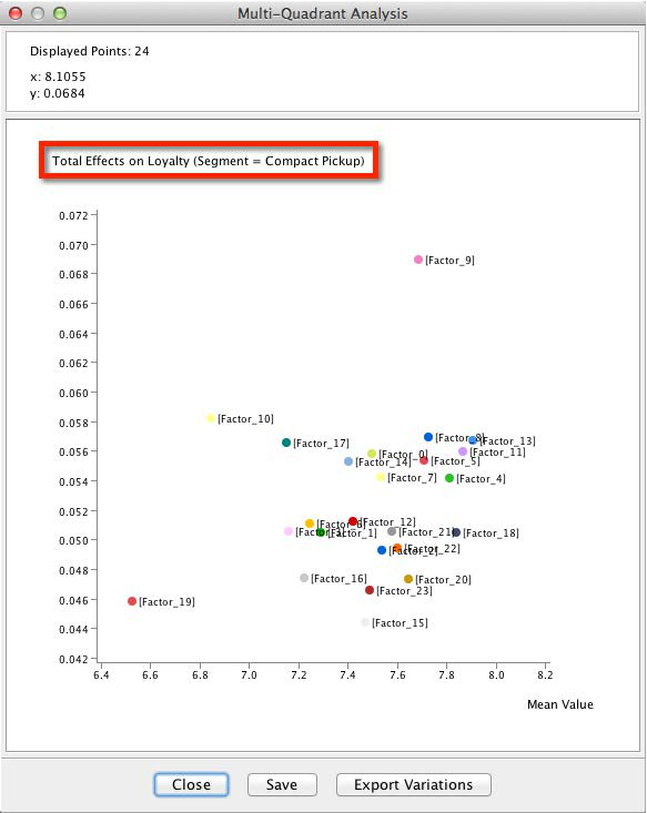
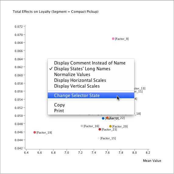
By default, the Breakout Variable’s first state is shown, in our case, Compact Pickup. To see the results of other segments, we right-click on the plot and pick Change Selector State.
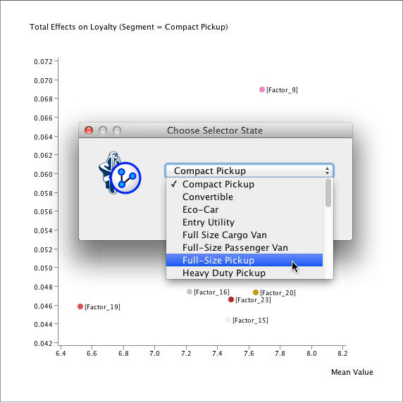
Full-Size Pickup Segment
For reasons explained in the introduction, we will now focus on the Full-Size Pickup segment.
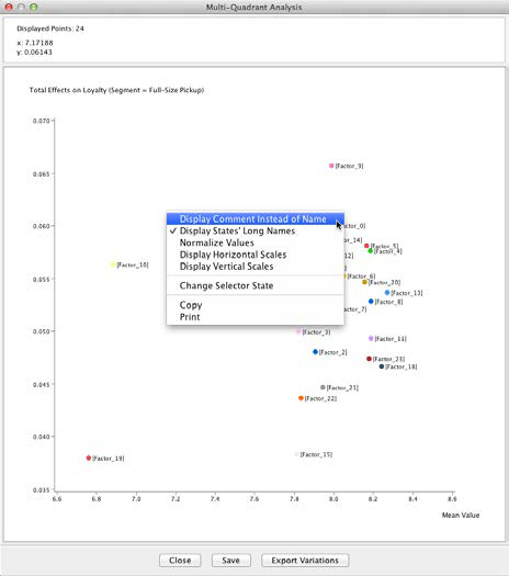
This plot allows immediate interpretation. The x-axis represents the mean satisfaction of Full-Size Pickup buyers with regard to the factors. The y-axis shows the Total Effect of each factor with regard to Loyalty. More specifically, the y-axis shows the value associated with a one-unit change in the respective factor. Casually speaking, we interpret this as the “importance” of a variable. For Full-Size Pickup, this means that Ability to Control Sound Quality is fairly unimportant for Loyalty. On the other hand, even though Affordable to Buy rates low on the x-axis, it rates fairly high on the y-axis, meaning it is rather important for Loyalty.
The following conceptual diagram shows a commonly used interpretation framework.
We should emphasize that we are interpreting factors, rather than manifest variables. Thus, the apparent “top driver” in the Full-Size Pickup plot, Length of Time Vehicle Will Remain Solid/Durable, is actually . For convenience, we apply the name of the node that contributes most strongly to this factor as its node comment. For reference, the manifest nodes associated with this factor are shown below.
In the Quadrant Plot, we can easily toggle between the factor name, i.e., , and the Node Comment via the contextual menu.
All the factors’ positions on the Quadrant Plot become even more meaningful in the context of other segments. Within the same Quadrant Plot window, we can hover over any of the factors to see how other segments compare on the selected attribute.
The following screenshot shows the positions of all segments with regard to Factor 17, which is labeled Length of Time Vehicle Will Remain Solid/Durable.
This plot would suggest, for instance, that the Full-Size Cargo Van segment has opportunities in this context. The Premium Convertible/Roadster segment, at the other end of the spectrum, might be in the “overkill” zone.
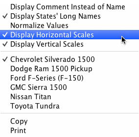
BayesiaLab offers a convenient way to see the relative position versus the segments. From the contextual menu, we can select Display Horizontal/Vertical Scales.
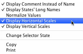
These scales show the range from the lowest to highest values. Additionally, a tick mark indicates the mean value of the respective attribute.
In the plot below, we show the Total Effect for Length of Time Vehicle Will Remain Solid/Durable for each segment. The intersection of the horizontal and vertical scales indicates the position of the Full-Size Pickup segment with regard to this variable.
This analysis can certainly help us to understand the general areas that are important for loyalty in the individual segments. However, it does not provide any insight into the specific opportunities for individual vehicle models. For this, we need to proceed to the next level of detail, i.e., the model level.
Multi-Quadrant Analysis (Segment ➔ Model)
During the earlier Multi-Quadrant Analysis, BayesiaLab generated one network file for each vehicle segment. We now open the network for the Full-Size Pickup, the focus of this study.
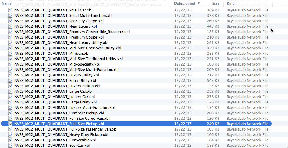
Although the structure of this segment-specific network is identical to that of the original network, all relationships between nodes, factors, and the target were re-estimated based on the subset of data corresponding to the Full-Size Pickup segment.
Relearning the Structure at the Market Level
As we move from the overall market into specific segments, and then models, we need to ask whether the structure learned at the market level will also hold true at the segment or model level.
In fact, we need to make a trade-off. We can retain the richer, more complex structure learned on the basis of the entire market, and simply reestimate the parameters. Alternatively, we can relearn the network structure on the much smaller dataset of the Full-Size Pickup segment. As opposed to the 71,200 cases for the entire market, we would then only have 2,003 observations [10] available for learning.
We hypothesize that the Full-Size Pickup segment has peculiarities that lead to structural differences versus the overall market. Consequently, we decide to relearn the network structure. The number of observations we have for this segment seems adequate to learn a reliable structure.
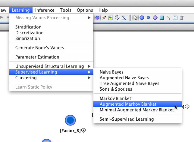
As before, we use the Augmented Markov Blanket algorithm: Learning > Supervised Learning > Augmented Markov Blanket.
[10] Count of unweighted observations.

We may find the resulting network a bit surprising as only a single arc is discovered, namely a connection between Affordable to Buy and Loyalty.
As we have not changed the default value, BayesiaLab used SC=1 for learning. Given the smaller amount of data available for this segment, we need to examine whether this is the appropriate value here.
Once again, we perform a Structural Coefficient Analysis: Tools > Cross Validation > Structural Coefficient Analysis.
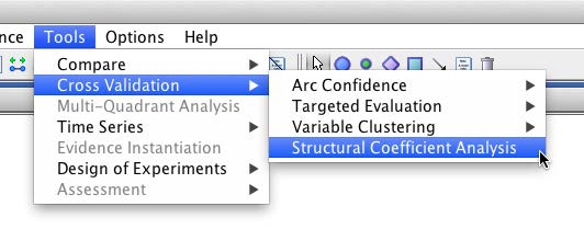
As a result, we obtain the now-familiar scree plot, which suggests that SC=0.6 is a reasonable value.
We set the Structural Coefficient accordingly:
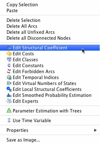
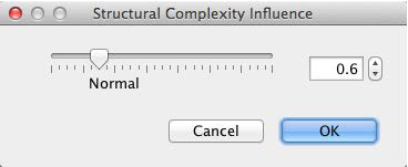
Once set, we proceed to relearning the network: Learning > Supervised Learning > Augmented Markov Blanket.
The resulting network now includes 7 factors. They appear fairly intuitive for this segment.
This is not to say that other factors do not matter. Rather, with the number of available observations, none other than the ones shown could be established with the given Structural Coefficient.
We now repeat the Target Mean Analysis: Analysis > Visual > Target Mean Analysis > Standard:
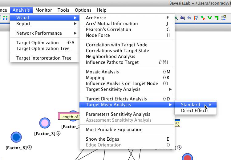
The resulting curves now show Loyalty as a function of the 7 factors in the network.
With the segment-specific network established, we can now proceed to the next level of detail, moving from Segment to Model.

For this purpose, we rerun the Multi-Quadrant Analysis and select Model as the Breakout Variable.
Furthermore, we must specify an output directory so we can subsequently analyze the model-specific networks.
Once again, we obtain a Quadrant Plot, now with Model as the selector.
As before, we can scroll through the individual states of the selector variable. By hovering over individual variables on the plot, we see the relative position of the models with respect to any factor.
The Display Horizontal/Vertical Scales command, which is available from the contextual menu of the Quadrant Plot, frames the range of competitors’ values.