Unsupervised Learning
The computational complexity of BayesiaLab’s Unsupervised Learning algorithms exhibits quadratic growth as a function of the number of nodes. However, the Maximum Weight Spanning Tree (MWST) is constrained to learning a tree structure (one parent per node), which makes it much faster than the other algorithms. More specifically, the MWST algorithm includes only one procedure with quadratic complexity, namely the initialization procedure that computes the matrix of bivariate relationships.
Given the number of variables in this dataset, we decide to use the MWST. Performing the MWST algorithm with a file of this size should only take a few seconds. Moreover, using BayesiaLab’s layout algorithms, the tree structures produced by MWST can be easily transformed into easy-to-interpret layouts. Thus, MWST is a practical first step for knowledge discovery. Furthermore, this approach can be useful for verifying that there are no coding problems, e.g., with variables that are entirely unconnected. Given the quick insights that can be gleaned from it, we recommend using MWST at the beginning of most studies.
We return to Modeling Mode F4 and select Menu > Learning > Unsupervised Structural Learning > Maximum Spanning Tree.
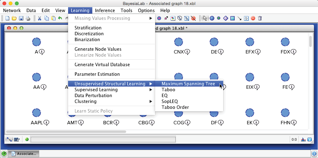
In addition to its one-parent constraint, MWST is also unique in that it is the only learning algorithm in BayesiaLab that allows us to choose the scoring method for learning, i.e., Minimum Description Length (MDL) or Pearson’s Correlation. Unless we are certain about the linearity of the yet-to-be-learned relationships between variables, Minimum Description Length is the better choice and, hence, the default setting.

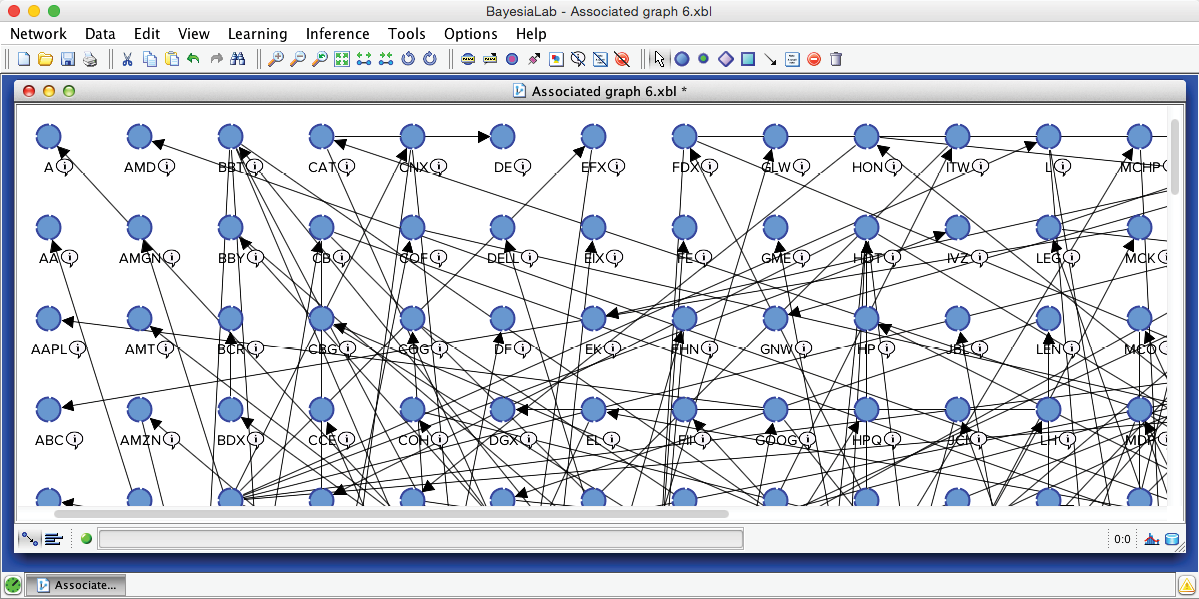
At first glance, the resulting network does not appear simple and tree-like at all.
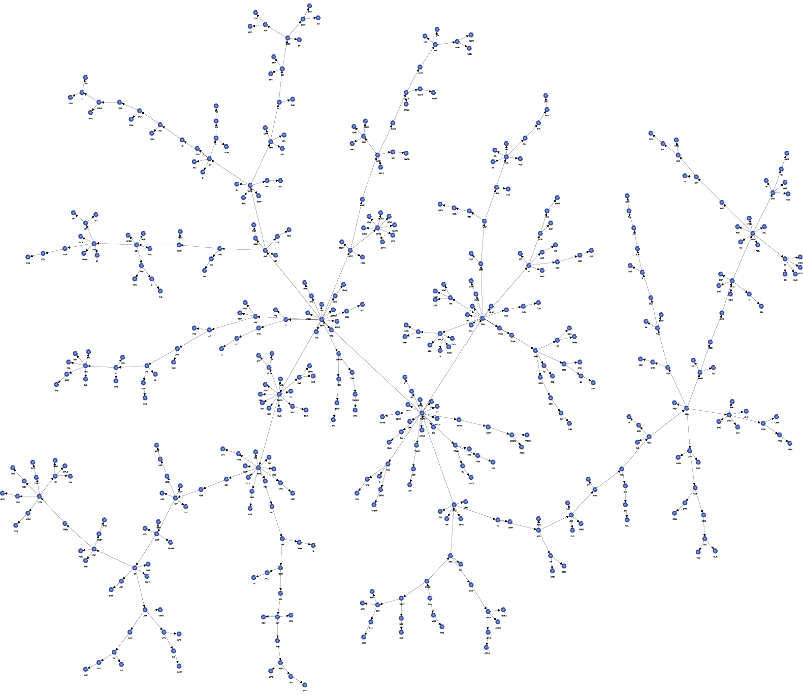
This can be addressed with BayesiaLab’s built-in layout algorithms. Selecting Menu > View > Automatic Layout (Shortcut: ) quickly rearranges the network to reveal the tree structure. The resulting reformatted Bayesian network can now be readily interpreted.
Network Analysis
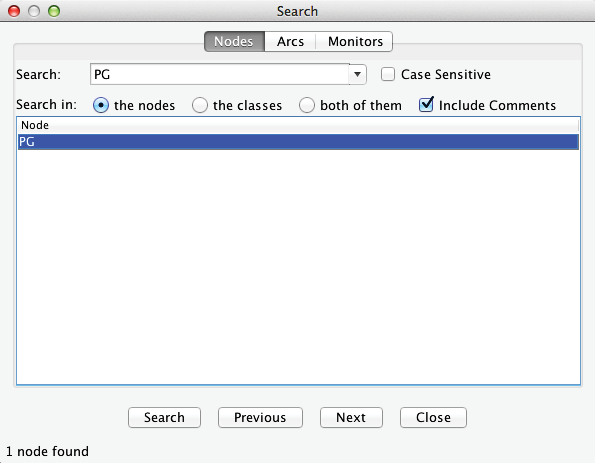
Let us suppose we are interested in Procter & Gamble (PG). First, we look for the corresponding node using the Search function (Ctrl+F). Note that we can search for the full company name if we check Include Comments. Furthermore, we can use a combination of wildcards in the search, e.g., ”*” as a placeholder for a character string of any length or ”?” for a single character.
Selecting PG from the listing search results makes the corresponding node flash for a few seconds so it can be found among the hundreds of nodes on the screen.
Once located, we can zoom in to see PG and numerous adjacent nodes.
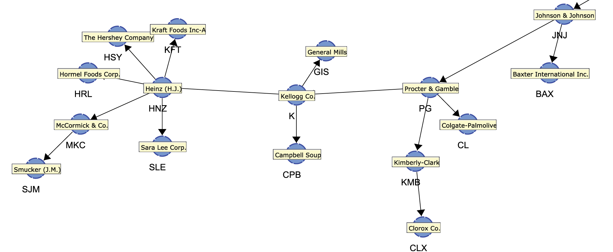
As it turns out, the “neighborhood” of Procter & Gamble contains many familiar company names, mostly from the consumer packaged goods industry. Perhaps these companies appear all too obvious, and one might wonder what insight we gained at this point. The chances are that even a casual observer of the industry would have mentioned Kimberly-Clark, Colgate-Palmolive, and Johnson & Johnson as businesses operating in the same field as Procter & Gamble. Therefore, one might argue similar stock price movements should be expected.
The key point here is that—without any prior knowledge of this domain—a computer algorithm automatically extracted a structure that is consistent with the understanding of anyone familiar with this domain.
Beyond interpreting the qualitative structure of this network, there is a wide range of functions for gaining insight into this high-dimensional problem domain. For instance, we may wish to know which node within this network is most important. In Chapter 6, we discussed the question in the context of a predictive model, which we learned with Supervised Learning. Here, on the other hand, we learned the network with an Unsupervised Learning algorithm, which means that there is no Target Node. As a result, we need to think about the importance of a node with regard to the entire network, as opposed to a specific Target Node.
We need to introduce a number of new concepts to equip us for the discussion about node importance within a network. We draw on concepts from information theory, which we first introduced in Chapter 5 under Information-Theoretic Concepts.
Arc Force
BayesiaLab’s Arc Force is computed by using the Kullback-Leibler Divergence, denoted by , which compares two joint probability distributions, and , defined on the same set of variables .
where is the current network, and is the exact same network as , except that we removed the arc under study.
It is important to note that Mutual Information and Arc Force are closely related (see Comparing Mutual Information and Arc Force). If the child node in the pair of nodes under study has no other parents, Mutual Information and Arc Force are, in fact, equivalent. However, the Arc Force is more powerful as a measure as it considers the network’s Joint Probability Distribution rather than only focusing on the bivariate relationship.
The Arc Force can be displayed directly on the Bayesian network graph. Upon switching to the Validation Mode F5, we select Menu > Analysis > Visual > Arc Force.
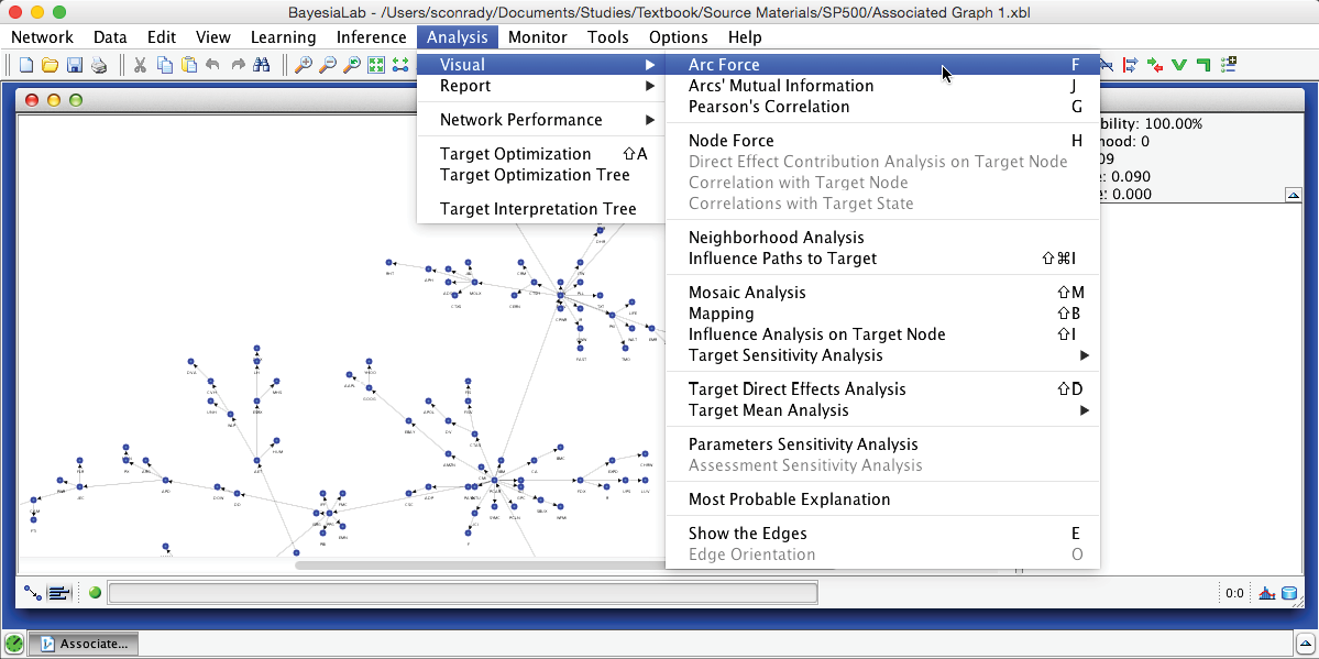
Upon activating Arc Force, we can see that the arcs have different thicknesses. Also, an additional control panel becomes available in the menu.

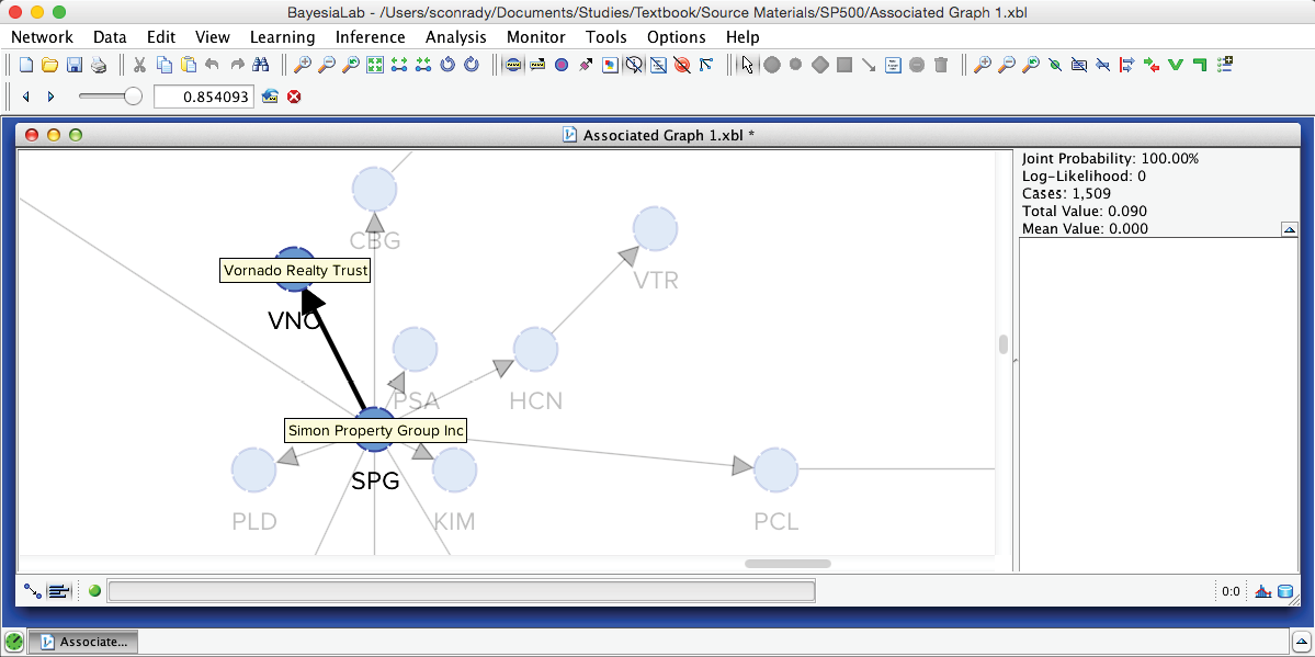
The slider in this control panel allows us to set the Arc Force threshold below which arcs and nodes will be grayed out in the Graph Panel. By default, it is set to 0, which means that the entire network is visible. Using the Previous and Next buttons, we can step through all threshold levels. For instance, by starting at the maximum and then going down one step, we highlight the arc with the strongest Arc Force in this network, which is between SPG (Simon Property Group) and VNO (Vornado Realty Trust).
Node Force
The Node Force can be derived directly from the Arc Force. More specifically, there are three types of Node Force in BayesiaLab:
- The Incoming Node Force is the sum of the Arc Forces of all incoming arcs.
- The Outgoing Node Force is the sum of the Arc Forces of all outgoing arcs.
- The Total Node Force is the sum of the Arc Forces of all incoming and outgoing arcs.
The Node Force can be shown directly on the Bayesian network graph. Upon switching to the Validation Mode F5, we select Analysis > Visual > Node Force.
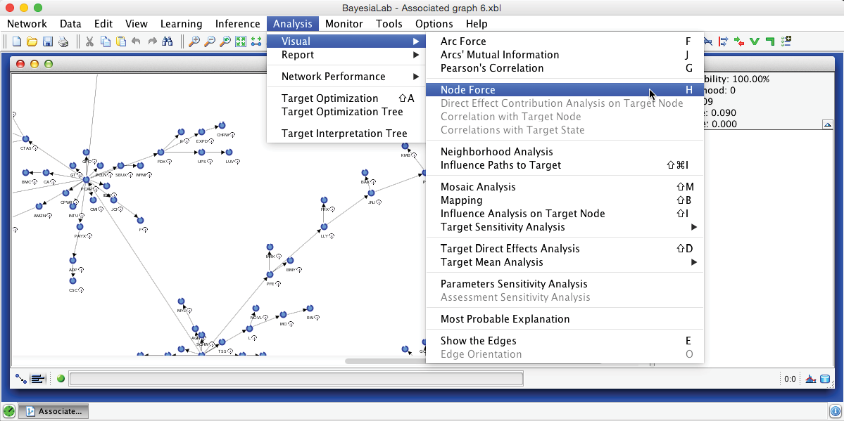
After starting Node Force, we have another additional control panel available in the menu.

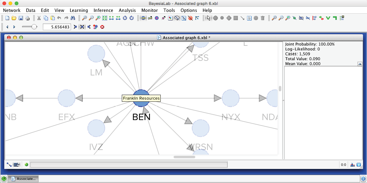
The slider in this control panel allows us to set the Node Force threshold below which nodes will be grayed out in the Graph Panel. By default, it is set to 0, meaning all nodes are visible. Conversely, by setting the threshold to the maximum, all nodes are grayed out. Using Previous and Next , we can step through the entire range of thresholds. This functionality is analogous to the control panel for Arc Force. For example, by starting at the maximum and then going down one step, we can find the node with the strongest Node Force in this network, which is BEN (Franklin Resources), a global investment management organization.
Node Force Mapping
This analysis tool also features a “local” Mapping function, which is particularly useful when dealing with big networks, such as the one in this example with hundreds of nodes. We refer to this as a “local” Mapping function in the sense of only being available in the context of Node Force Analysis, as opposed to the “general” Mapping function, which is always available within the Validation Mode F5 as a standalone analysis tool (Menu > Analysis > Visual > Mapping).
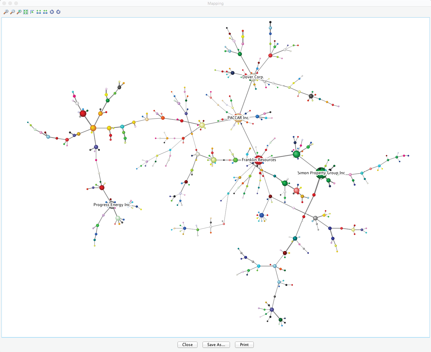
We launch the Mapping window by clicking the Mapping icon on the control panel to the right of the slider. In this network view, the size of the nodes is directly proportional to the selected type of Node Force (Incoming , Outgoing , Total ). The width of the links is proportional to the Arc Force. Changing the threshold values (with the slider, for example) automatically updates the view.
Choosing Static Font Size from the Context Menu and then, for instance, reducing the threshold by four more steps reveals the five strongest nodes while maintaining an overview of the entire network.
