Delays in Scheduled Flight Departures
This example uses Hellixia to analyze factors associated with delays in scheduled flight departures.
It shows how Hellixia can generate Causal Bayesian Networks (CBNs) that organize candidate drivers of flight delays, including weather, logistics, operations, and related constraints.
The following sections describe the semantic-analysis workflow and the construction of causal networks in BayesiaLab.
Semantic and Hierarchical Semantic Networks
First, we will perform a semantic analysis of the domain to obtain an overview of the key concepts and variables within the aircraft delay domain.
For our analysis of “Delays in scheduled flight departures”, we start by building a semantic network, followed by a hierarchical semantic network, similar to our previous workflows (for example, as demonstrated with Hamlet). This process is essential for mapping the semantic landscape surrounding flight delays, providing a solid foundation for understanding the underlying dynamics of this issue.
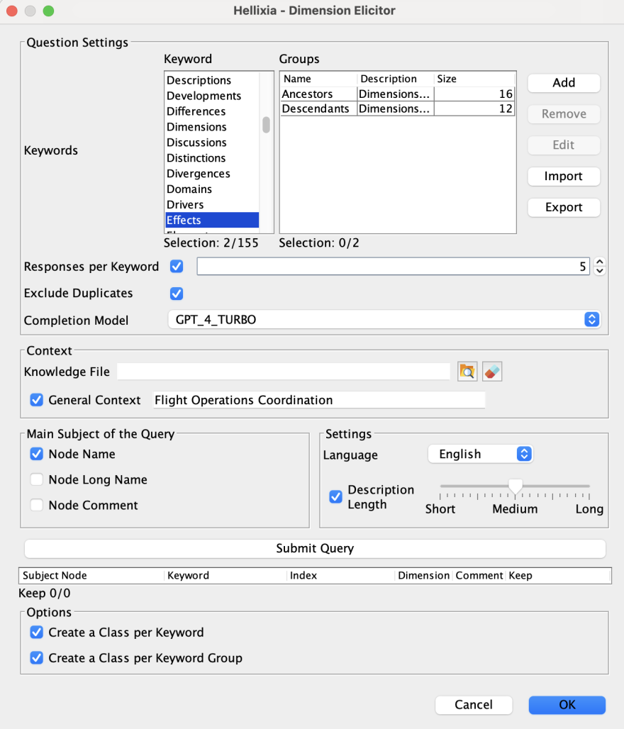
Create a node entitled “Delays in scheduled flight departures” and use Hellixia’s Dimension Elicitor with two distinct groups of keywords: Ancestors and Descendants. This approach allows us to explore what leads to and results from flight delays.
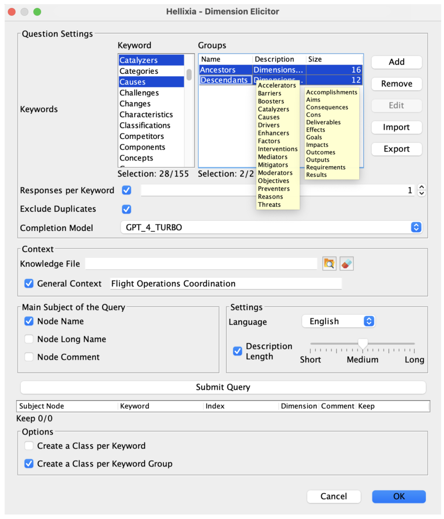
Carefully examine the dimensions provided by Hellixia, removing anything that seems extraneous or irrelevant to the analysis.
Exclude “Delays in scheduled flight departures” and run the Embedding Generator on the remaining nodes. This step is crucial to understanding the semantic relationships linked to their names and comments.
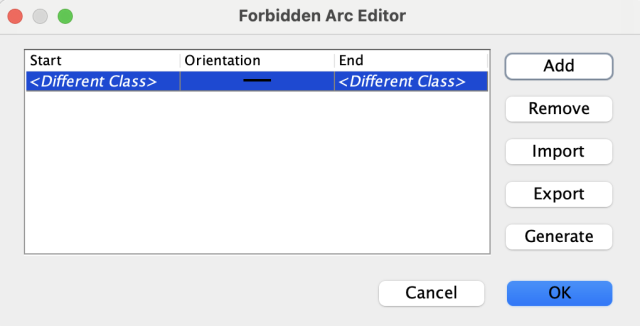
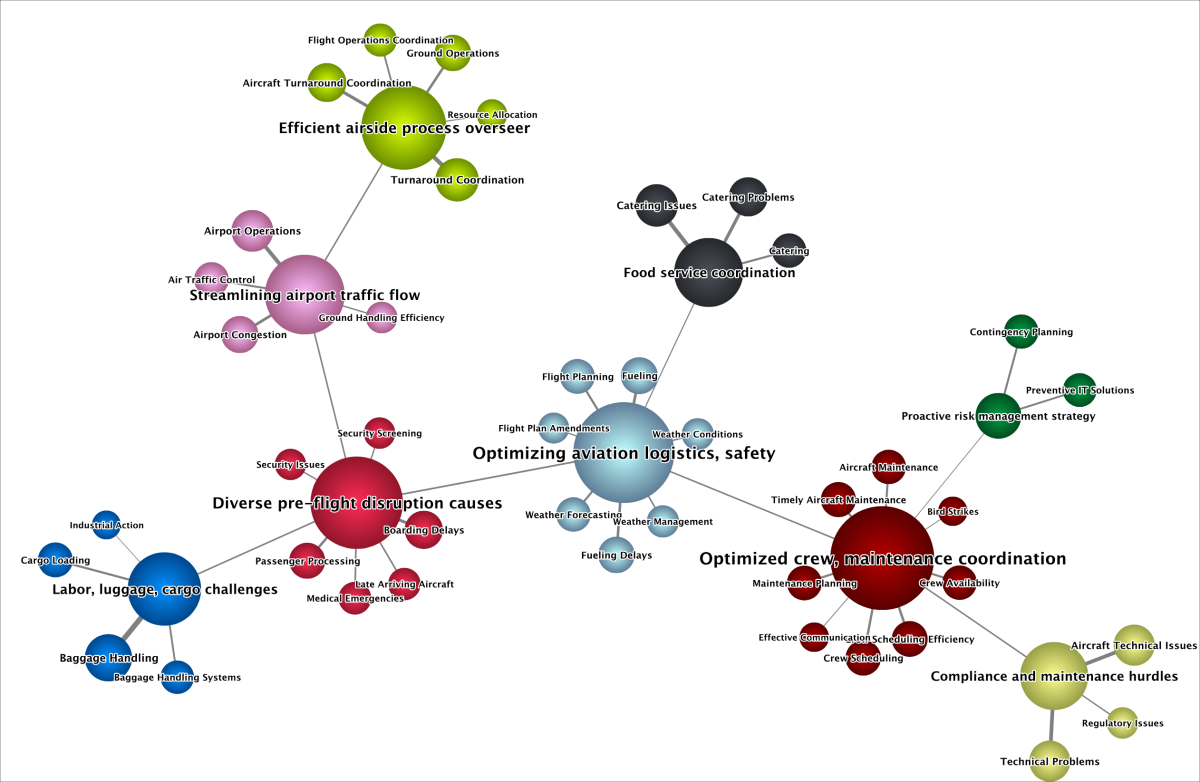
Use the two large node sets, “Ancestors” (42 nodes) and “Descendants” (69 nodes), to learn a separate network for each group. To do this, define specific constraints that prohibit relationships between nodes that do not belong to the same class.
Run the Maximum Weight Spanning Tree algorithm to find the most significant semantic relationships between nodes.
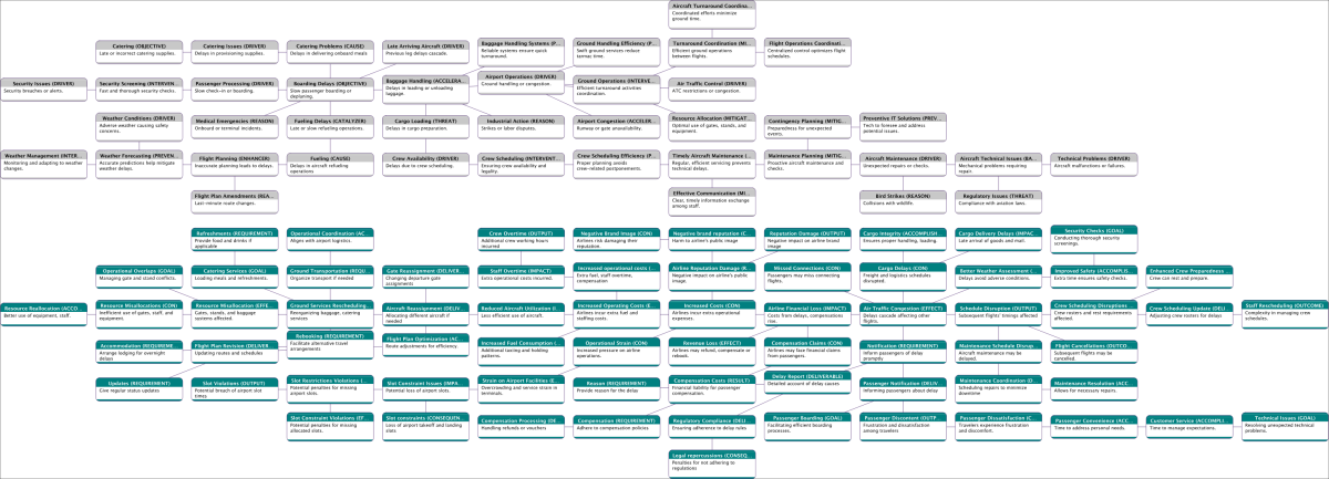
To improve interpretability, change the node styles to Badges, displaying the Node Comments.
Run the Dynamic Grid Layout to position the nodes on the graph. This algorithm is not deterministic, resulting in random orientations - vertical, horizontal or mixed. As a result, we may have to apply this layout several times to get a configuration that matches the intended presentation.
Switch to Validation Mode F5 and opt for the Skeleton View. Since the network does not represent causal relationships, the Skeleton View is useful because it shows the connections between nodes while avoiding arrowheads that normally indicate arc direction.
Run Variable Clustering. This step categorizes variables that are similar, grouping them based on the semantic relationships identified between them.
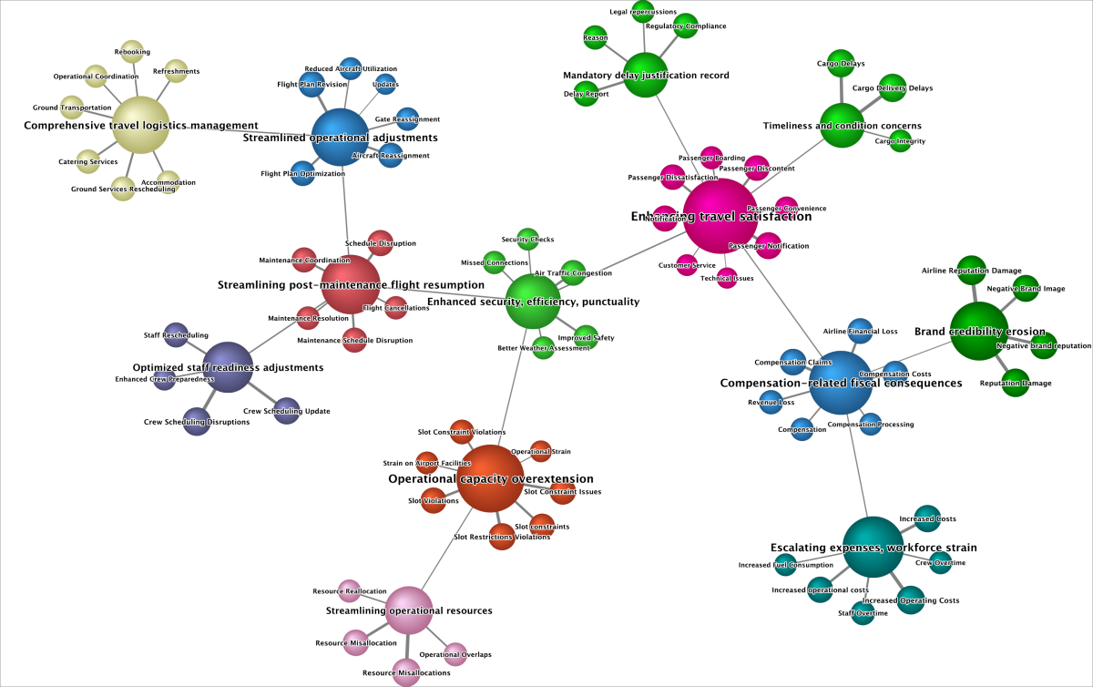
We can now proceed with creating two hierarchical semantic networks.
Access the Class Editor and then run the Class Description Generator. This generates descriptive names for the factors we’re examining.
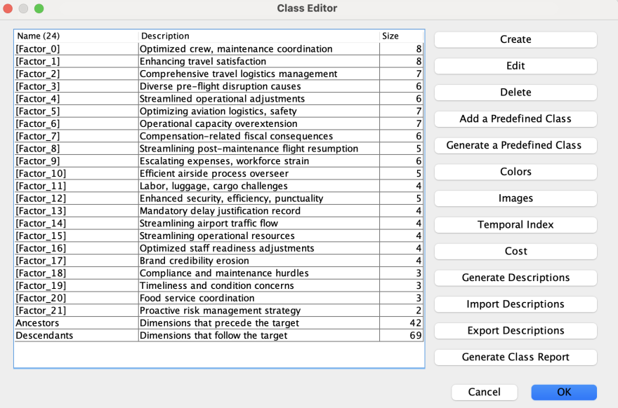
Use the Export Descriptions function to save the newly created factor descriptions.
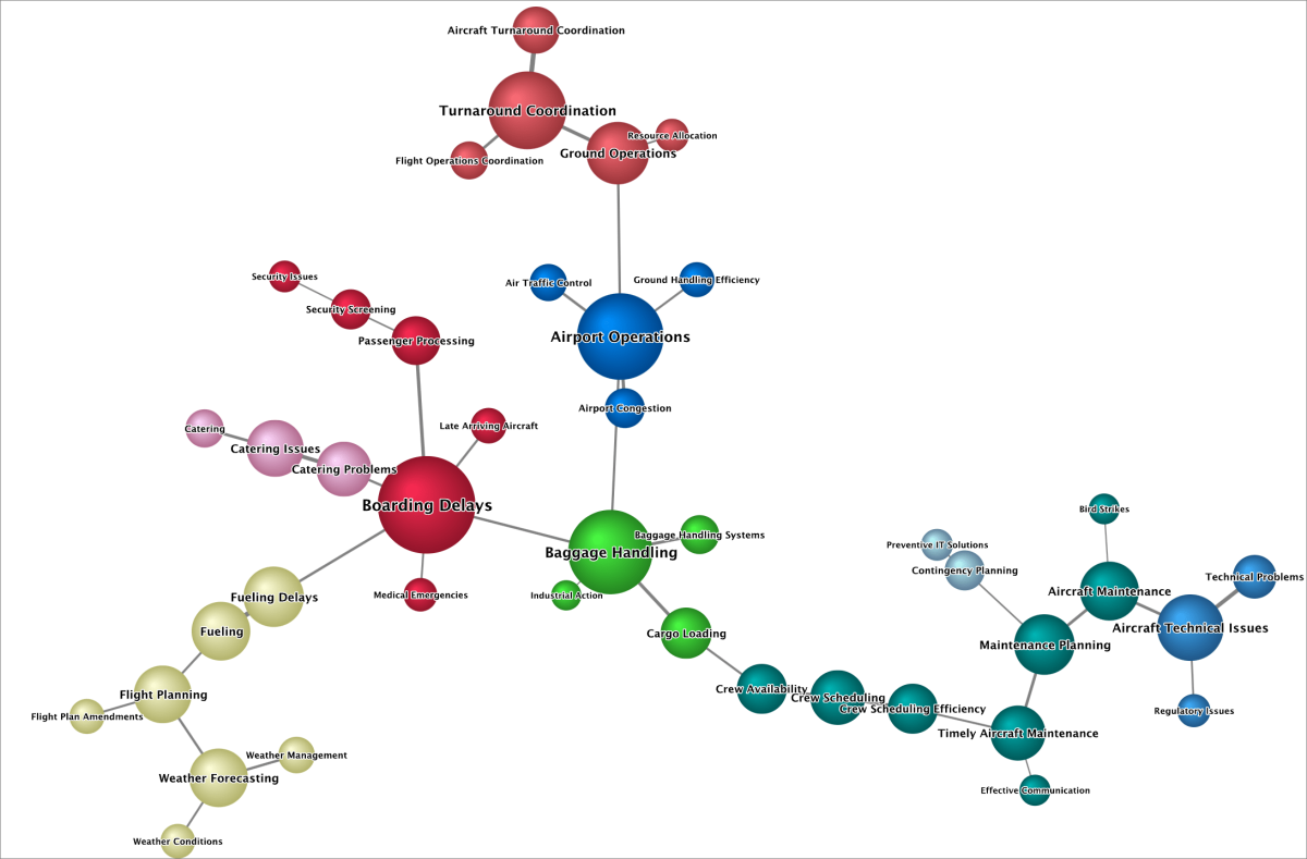
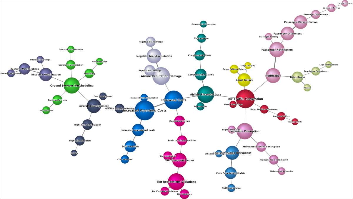
Switch back to Modeling Mode F4 and conduct Multiple Clustering to create latent variables.
Run the Taboo algorithm for structural learning, and make sure that the Delete Unfixed Arcs option is selected.
Utilize the descriptions previously exported as a Dictionary to rename the latent variables, adding clarity to the model.
Go back to Validation Mode F5 and run the Node Force analysis, which helps us understand the dynamics and strength of the connections within the network.
Causal Networks
Having established an overall understanding of the domain via semantic networks, we’re now ready to move forward with the construction of causal Bayesian networks, taking advantage of the capabilities introduced in Hellixia as part of BayesiaLab version 11.2.
Low Complexity Causal Network Created Using the Causal Network Generator
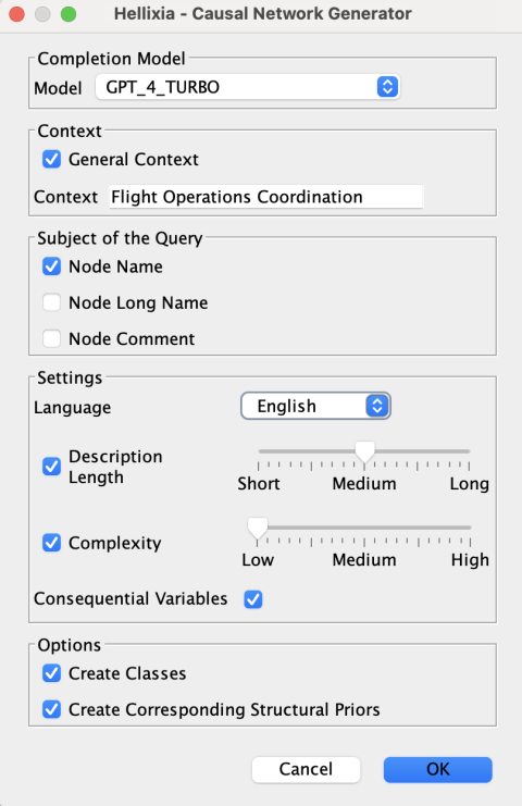
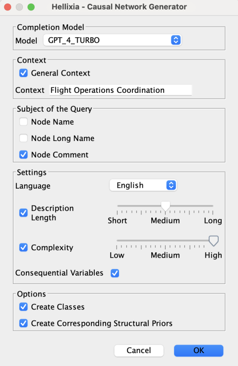
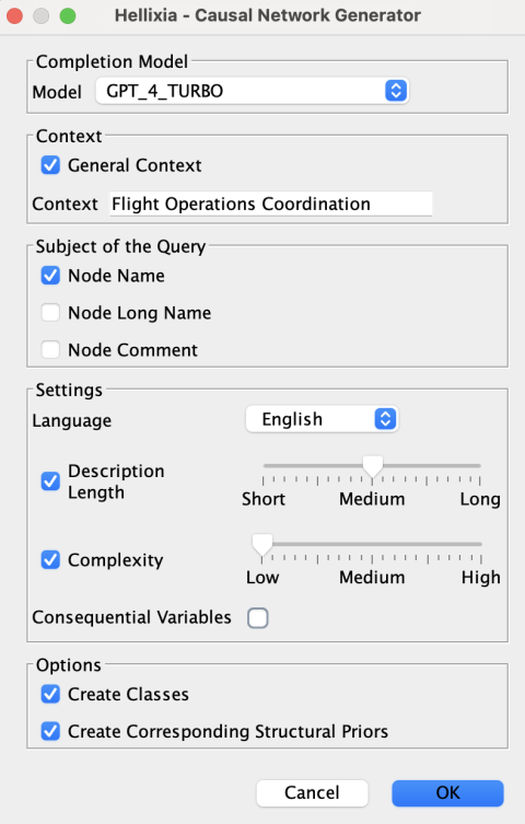
Create a node named Delays in Scheduled Flight Departures and use the Causal Network Generator feature.
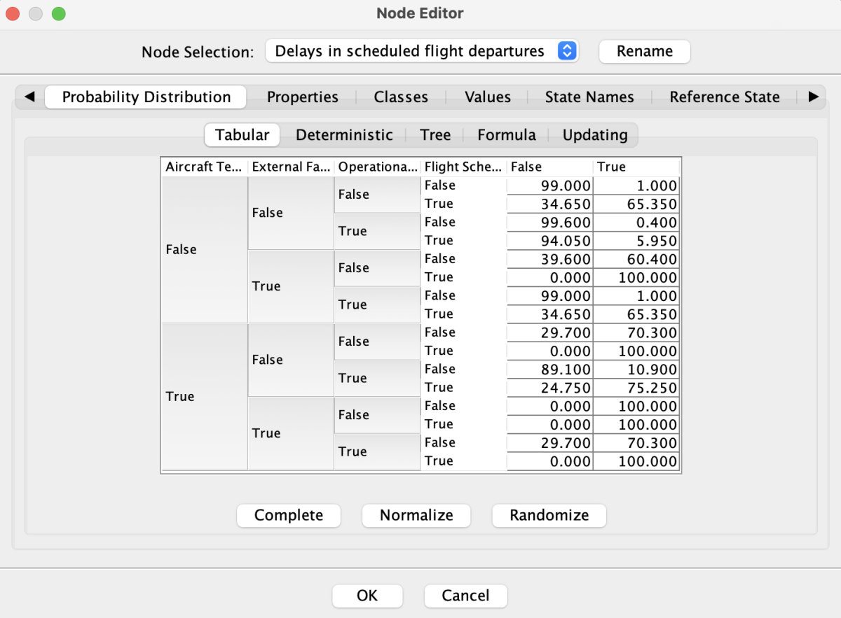
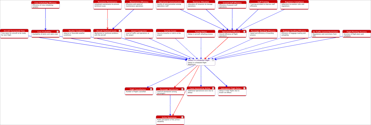
After one or two minutes, depending on the complexity of the prompt, review the small but fully specified causal Bayesian network, including both graph and probabilities. The network features directed arcs to signify causal relationships, with each arc accompanied by a succinct explanation of its causal link and an estimate of the effect, scaled from -100 (shown in red) to 100 (shown in blue).
To differentiate nodes by depth using different colors, first run the Edit Class function. Next, select Generate a Predefined Class - Depth. Then select the four depth classes that have been created and apply the Colors - Associate Random Colors with Classes function to assign distinct colors to each class.
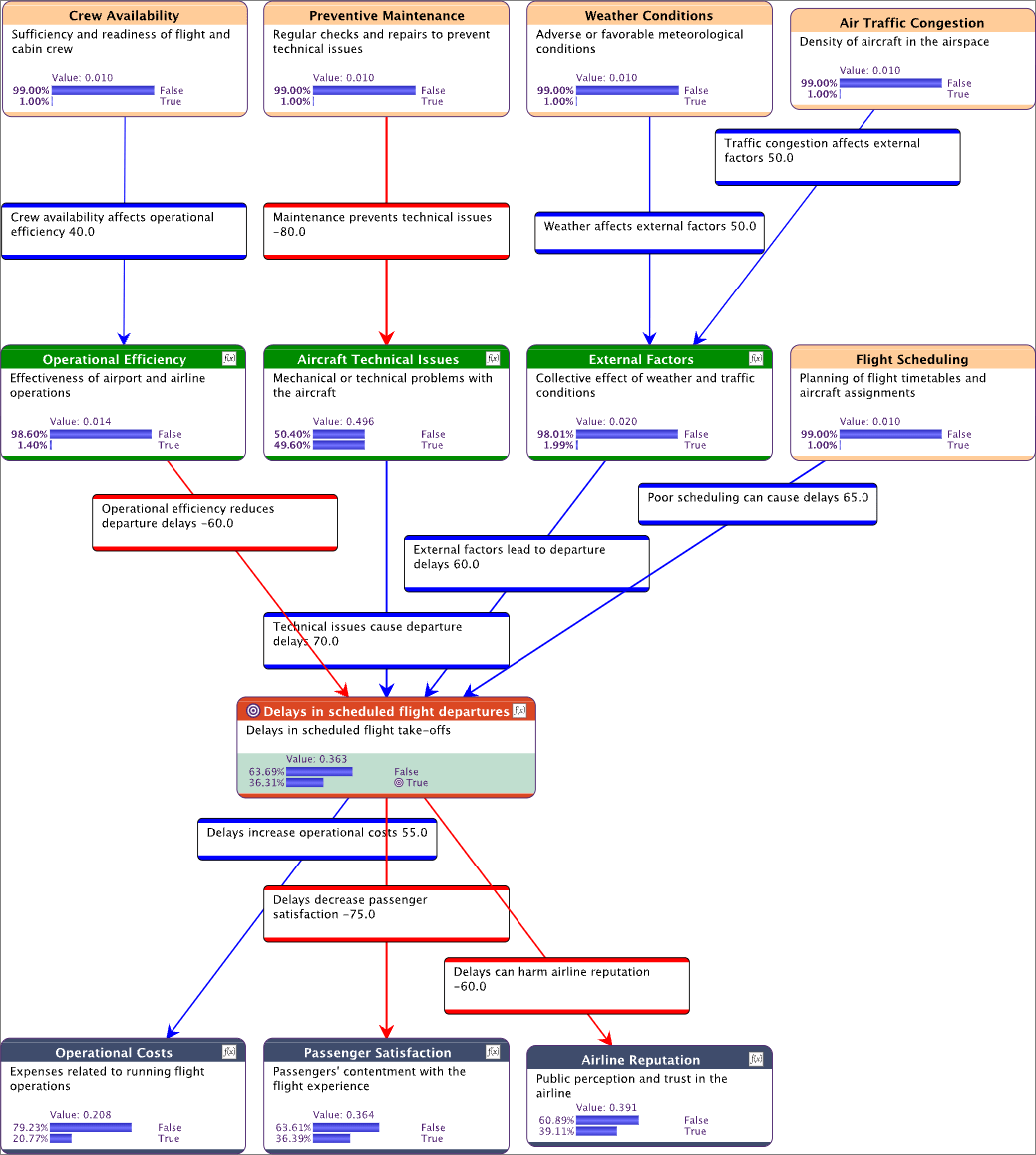
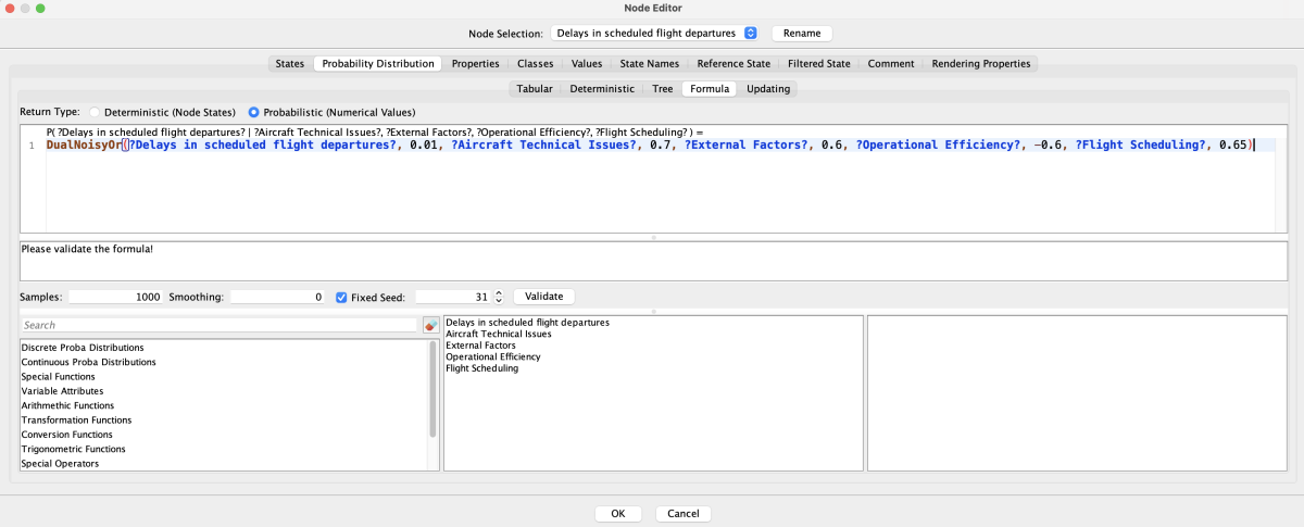
Inspect the nodes marked with an icon representing a function. These nodes are parameterized using BayesiaLab’s new DualNoisyOr() formula, which integrates both positive and negative interactions between Boolean variables, corresponding to the causal effects returned by Hellixia.
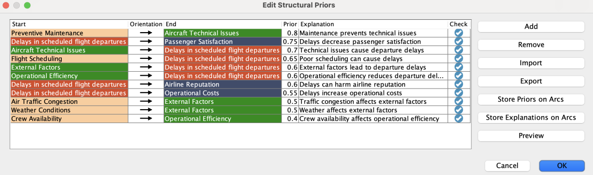
Review the Structural Priors made available by selecting the Create Corresponding Structural Priors option in the Causal Network Generator wizard. The value of each prior is derived from the absolute value of the causal effect returned by Hellixia, and the explanation provided for each prior corresponds to the description of its causal relationship. These structural priors can then be used later for network learning when relevant data becomes available.
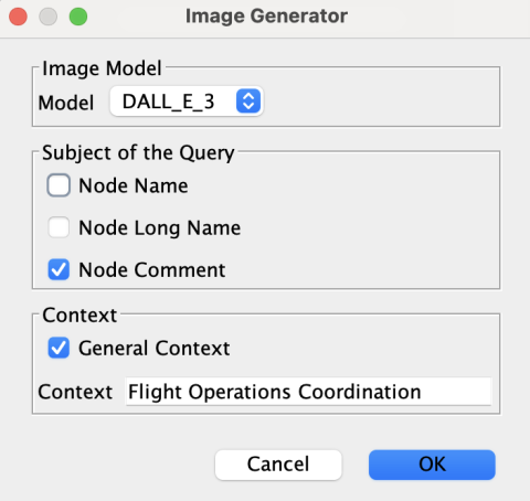
To finalize this first causal network, use the Hellixia Image Generator to create unique icons for each node, based on the comment.
Higher Complexity Causal Network Created Using the Causal Network Generator
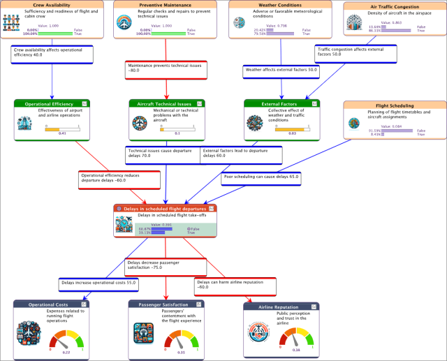
Move on to the creation of a more complex causal network by setting Complexity to High.
Examine the automatically generated network in depth. For example, Fueling Delays is identified as a direct cause. Aircraft Turnaround Time is also identified as a direct cause. This leads to the hypothesis that Fueling Delays could be a direct cause of Aircraft Turnaround Time, which would have an indirect effect on flight delays.
To verify this hypothesis, select the two nodes, Fueling Delays and Aircraft Turnaround Time, and apply the Hellixia Pairwise Causal Link feature. This helps ascertain the nature of the causal relationship between these variables.
Review the validated causal relationship and the updated conditional probability distribution of Aircraft Turnaround Time. This update incorporates a DualNoisyOr() function with a coefficient of 0.75, reflecting the quantified impact of Fueling Delays on Aircraft Turnaround Time. Following this update, remove the direct link from Fueling Delays to Delays in Scheduled Flight Departures and adjust the DualNoisyOr() formula to reflect this change in the network’s structure.
To examine causes of causes, select the relevant node and run the Causal Network Generator again, this time on Fueling Delays.
Review the newly added nodes and relationships. Three relationships are incorrectly marked as negative, contrary to the descriptions in their respective link comments. To rectify this, change the color of these links to accurately reflect their positive nature and update the DualNoisyOr() formula of Operational Efficiency.
Low Complexity Causal Network Created Using the Causal Relationship Finder
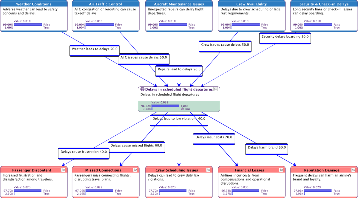
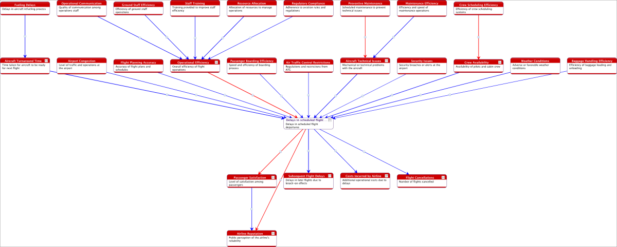
To conclude our analysis, we’re going to build a final causal network, this time using the Causal Relationship Finder function. Unlike the Causal Network Generator, which added new nodes for creating the network, this feature works directly with selected nodes. To begin with, we use the Dimension Elicitor tool to identify the 5 main Causes and 5 main Effects associated with Delays in Scheduled Flight Departures.
Use the Dimension Elicitor tool to identify the 5 main Causes and 5 main Effects associated with Delays in Scheduled Flight Departures.
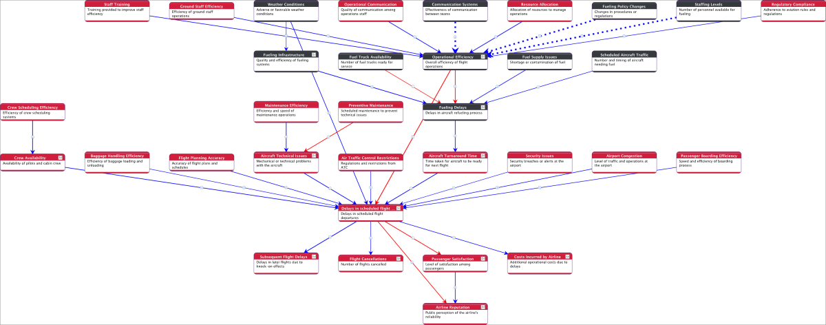
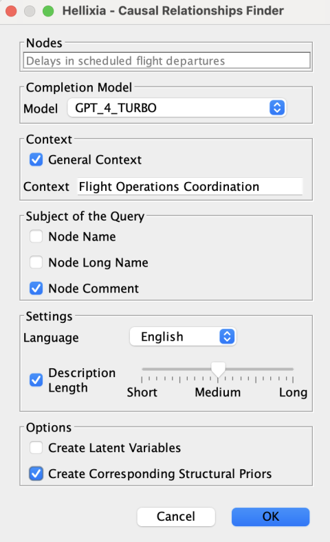
Select the 10 causes and effects, along with the Delays in Scheduled Flight Departures node. With these nodes selected, run the Hellixia Causal Relationships Finder to create the network.
Review the resulting bow-tie network structure.