Naive Bayes Network
Rather than computing the relationships individually for each pair of nodes, we ask BayesiaLab to estimate a Naive Bayes network. A Naive Bayes structure is a network with only one parent, the Target Node, i.e., the only arcs in the graph are those directly connecting the Target Node to a set of nodes. By designating SalePrice as the Target Node, we can automatically compute its Mutual Information with all other available nodes.
For the node SalePrice, we select Node Context Menu > Set as Target Node. Alternatively, we can double-click the node while pressing T.
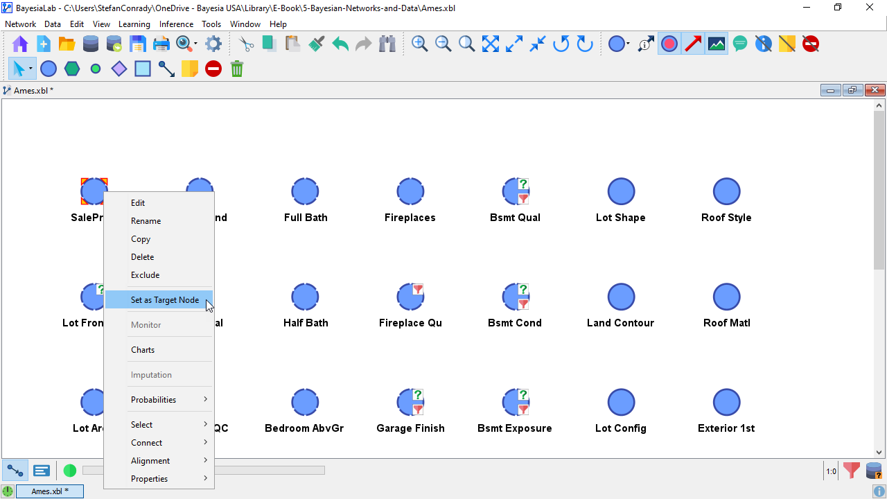
The special status of the Target Node is highlighted by the bullseye symbol . We can now proceed to learn the Naive Bayes network: Select Menu > Learning > Supervised Learning > Naive Bayes.
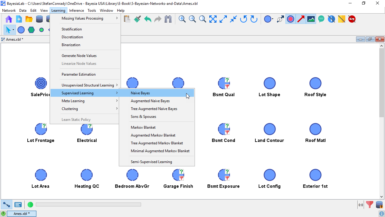
Strictly speaking, we are not learning a network in the true sense of machine learning. Rather, we are specifying a naive structure, i.e., arcs from the Target Node to all other nodes, and then estimating the parameters.
Due to its simplicity, the Naive Bayes network is presumably the most commonly used Bayesian network. As a result, we find it implemented in many software packages. For instance, the so-called Bayesian anti-spam systems are based on this model.
However, it is important to note that the Naive Bayes network is merely the first step towards embracing the Bayesian network paradigm.
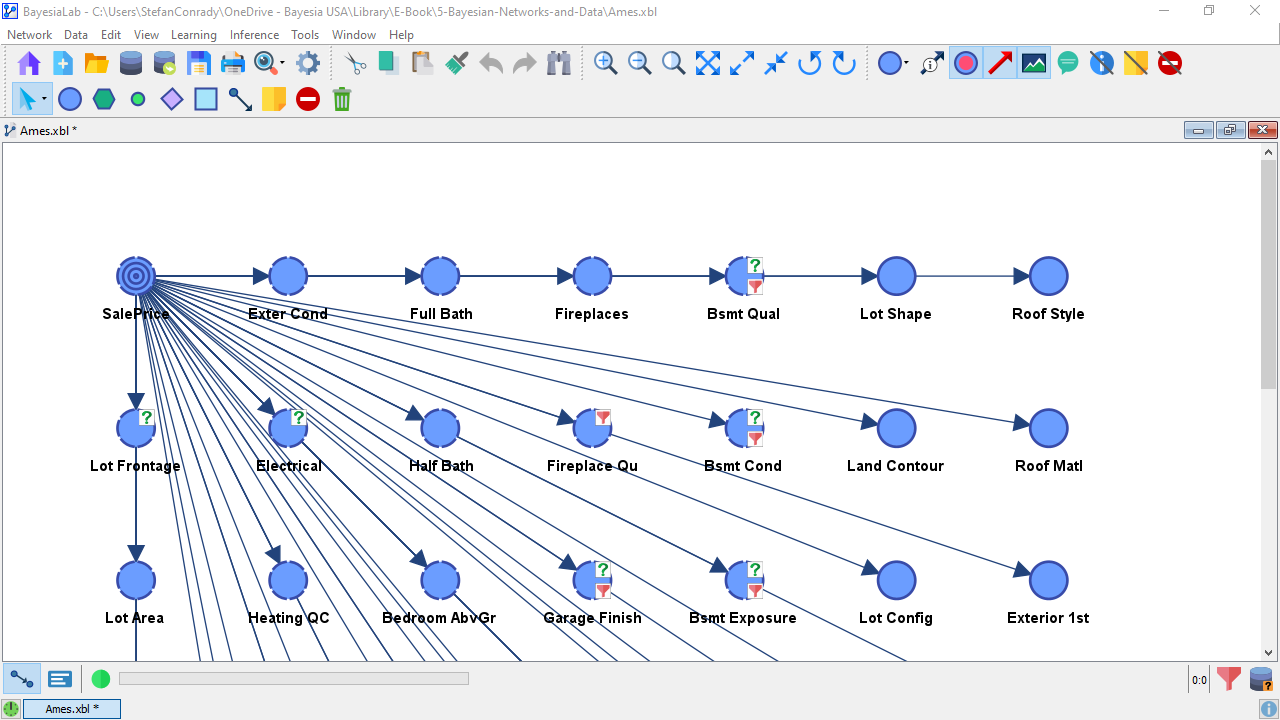
Now we have the network that allows computing the Mutual Information between all nodes.
We switch to Validation Mode F5 and select Menu > Analysis > Visual > Overall > Arc > Mutual Information.
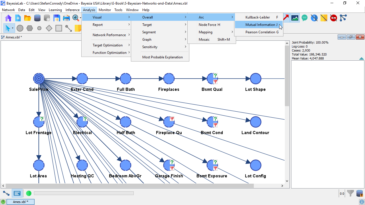
The different levels of Mutual Information are now reflected in the thickness of the arcs.
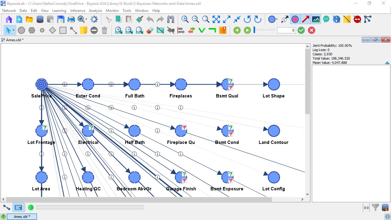
However, given the grid layout of the nodes and the overlapping arcs, it is difficult to establish a rank order of the nodes in terms of Mutual Information. To address this, we adjust the layout and select Menu > View > Layout > Radial Layout.
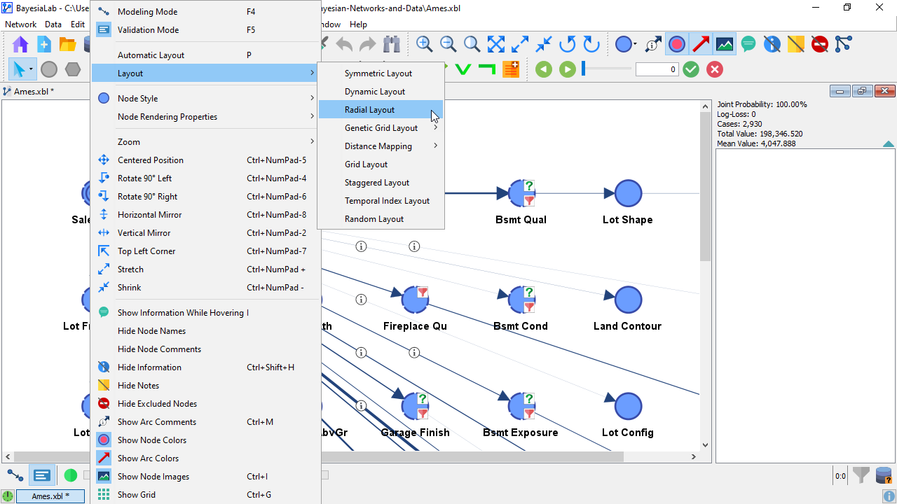
This generates a circular arrangement of all nodes with the Target Node, SalePrice, in the center. Clicking the Stretch icon repeatedly, we expand the network to make it fit into the available screen space widthwise.
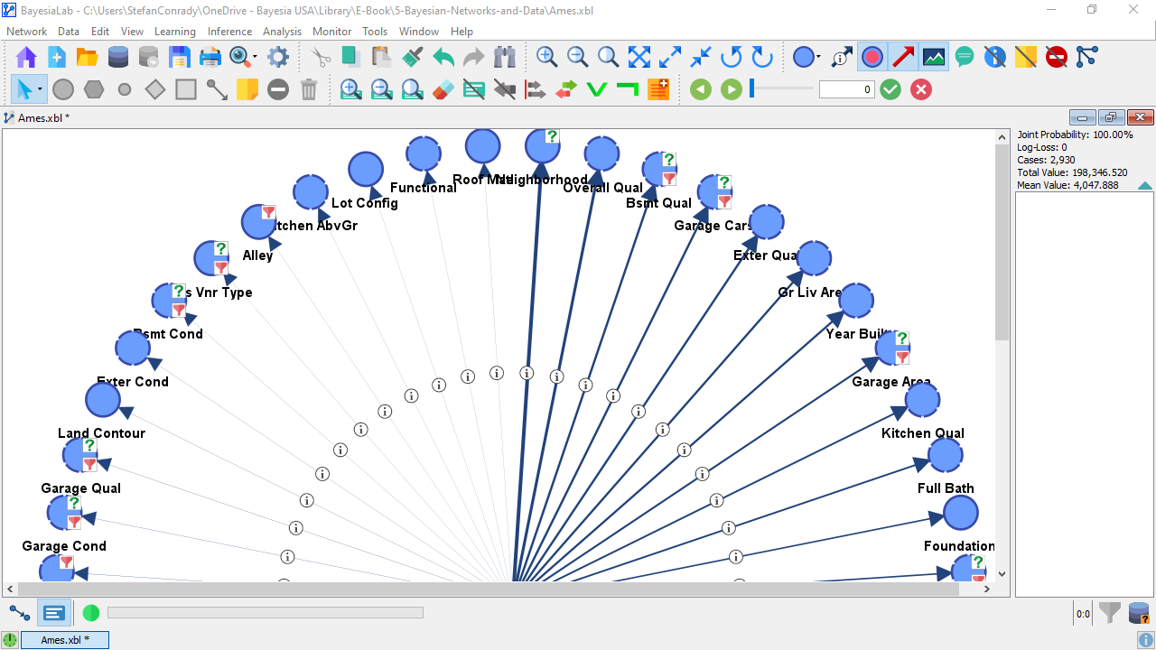
Also, having run the Radial Layout while the Arc Mutual Information function was still active, the arcs and nodes are ordered clockwise from strongest to weakest Mutual Information.
To improve the interpretability further, we select Menu > View > Hide Information. Alternatively, we click the Hide Information icon in the Toolbar. This removes the information icons from the arcs. Their presence indicates that further information would be available to display, e.g., the numerical values of the Mutual Information of each arc.
The following standalone graphic highlights the order of the arcs and nodes in this Naive Bayes network:
This illustration shows that Neighborhood provides the highest amount of Mutual Information and, at the opposite end of the range, RoofMtl (Roof Material) the least.
As an alternative to this visualization, we can run a report Main Menu > Analysis > Report > Relationship:
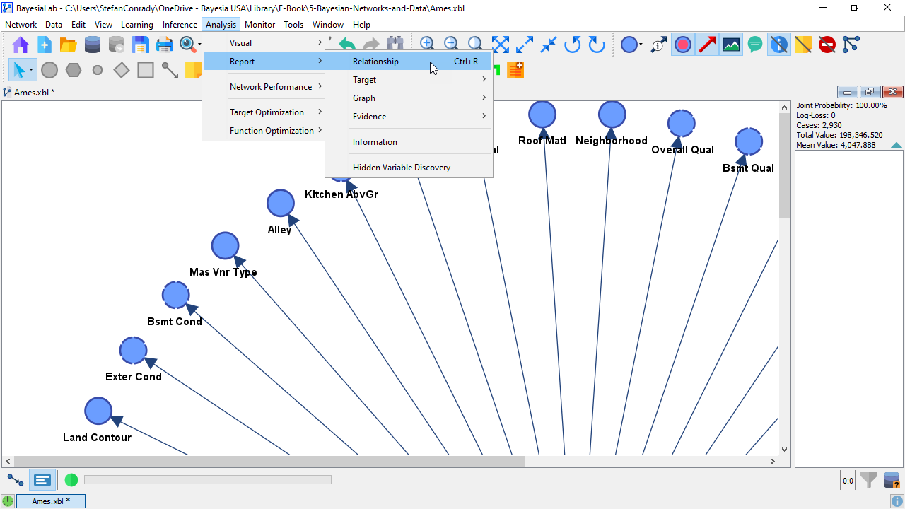
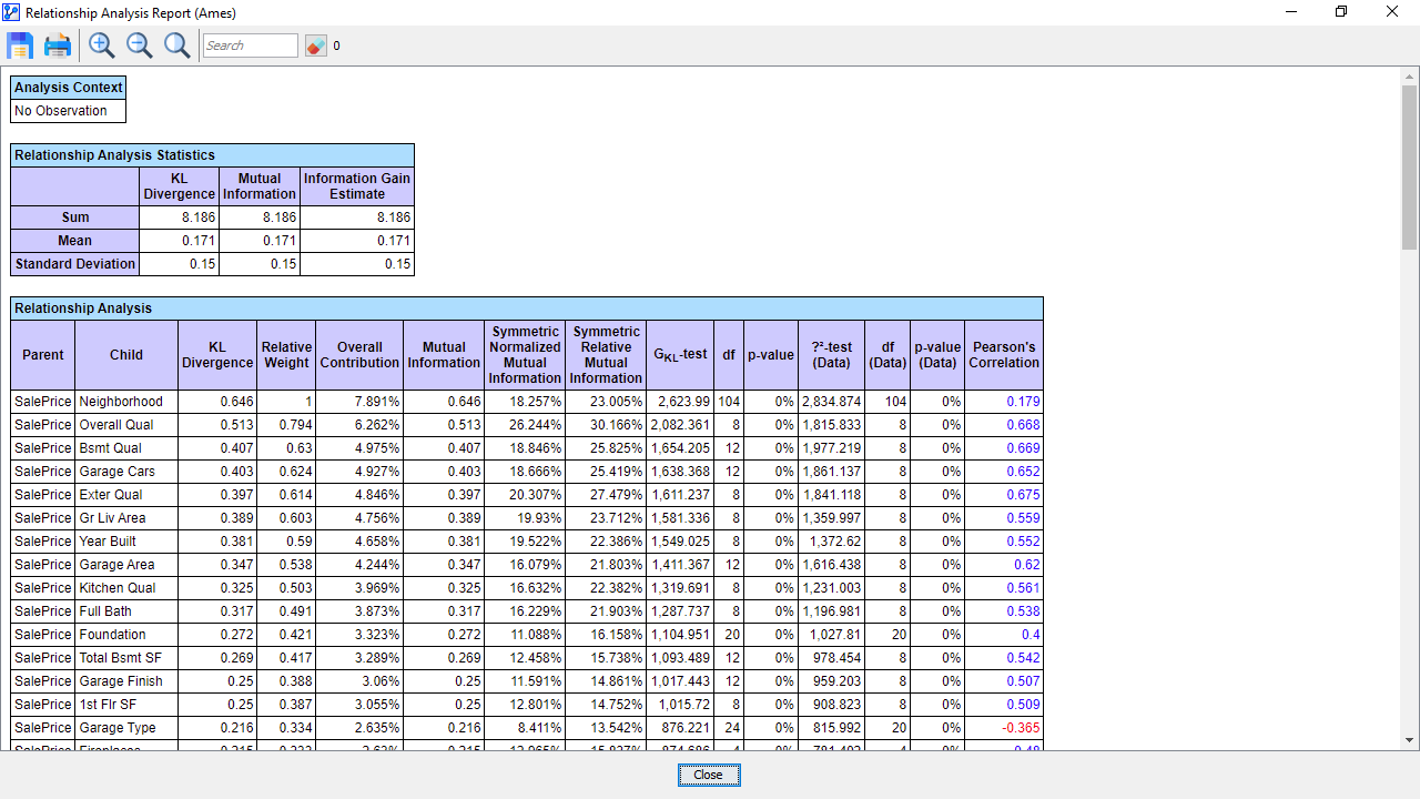
Wouldn’t this report look the same if computed based on correlation? In fact, the rightmost column in this Relationship Analysis Report shows Pearson’s Correlation for reference. As we can see, the order would be different if we chose Pearson’s Correlation as the main metric.
So, what have we gained over correlation? One of the key advantages of Mutual Information is that it can be computed—and interpreted—between numerical and categorical variables without any variable transformation. For instance, we can easily compute the Mutual Information, such as between the Neighborhood and SalePrice. The question regarding the most important predictive variable can now be answered. It is Neighborhood.
Now that we have established the central role of Entropy and Mutual Information, we can apply these concepts in the next chapters for machine learning and network analysis.
