Example: Augmented Simpson’s Paradox
Now that we have seen how to estimate the Average Causal Effect by manually interacting with the BayesiaLab’s Monitors, with both Graph Surgery and Likelihood Matching, we will use the BayesiaLab’s Direct and Total Effect functions to compute causal effects automatically for a set of variables. But first, we present a slightly more complex version of Simpson’s Paradox to illustrate these features (see Example: Simpson’s Paradox).
Augmented Simpson’s Paradox
Our updated story contains four additional dimensions:
- Treatment Availability: the treatment is not always available;
- Side Effects: the treatment may produce severe side effects;
- Efficacy: some patients do not respond to the drug;
- Litigation: the families of patients who died may sue the pharmaceutical company that had provided the treatment.
The manually designed CDAG shown below describes this new domain qualitatively:
Next, we describe the quantitative part of the domain. First, we state that Treatment Availability is 75%. We also assume that the treatment may have Side Effects, which are much more frequent for females. The following conditional probability table quantifies this direct causal dependency on Gender:
Patients decide whether or not to take the treatment based on two criteria, Treatment Availability and Side Effects. The dependencies are described in the following table. It states that if the treatment is unavailable, patients cannot have the treatment, which is deterministic (and obvious). However, if the treatment is available, those patients who do not have any risk of experiencing side effects will always choose the treatment, while those at risk will be unlikely to submit to the treatment:
Furthermore, the Efficacy of the treatment depends on Drug Administration plus some hidden factors that render the treatment ineffective in 20% of patients:
The Target Node, Outcome, is defined by Gender and Efficacy. In this context, “not recovered” means that the patient died — hence the grim illustration attached to the icon.
Finally, half of the families of those patients who took the treatment and died are pursuing litigation. More specifically, these families are suing the pharmaceutical company that provided the treatment.
Path Analysis
We now list the paths between each variable and the target variable Outcome by using Menu > Analysis > Visual > Graph > Influence Paths to Target.
The causal paths are highlighted in blue (), and the non-causal paths (i.e., paths with at least one “backward” arrow ←) are shown in pink ():
Recall the Adjustment Criterion, which stipulates that we must keep all of a variable’s causal paths to the target variable open and simultaneously block all its non-causal paths for estimating its causal effect.
Graph Surgery
To illustrate BayesiaLab’s Total and Direct Effects functions with Graph Surgery, we set all nodes but Outcome to Intervention Mode.
Notice the arrow symbols (→) in the badges of the nodes that are set to Intervention Mode.
Average Causal Effect
Before using BayesiaLab’s automated tools for computing causal effects, we manually estimated the causal effect of our main variable of interest, Drug Administration, by using the Monitors.
Setting a piece of Evidence in Intervention Mode simulates an intervention on Drug Administration and mutilates the graph, as shown below, which meets the Adjustment Criterion by blocking the non-causal path (cf. Path Analysis, #6).
The Average Causal Effect of Drug Administration on Outcome, mediated by Efficacy, is -0.08.
Total Effects
We have seen in Chapter 8 that BayesiaLab estimates Total Effects as the derivatives of Total Effect Curves. These curves are based on the Posterior Mean Values of the Target Node given Mean Values from the interval of the variable under study. While the variables are in Intervention Mode, the Posterior Mean Values are computed based on the mutilated graph.
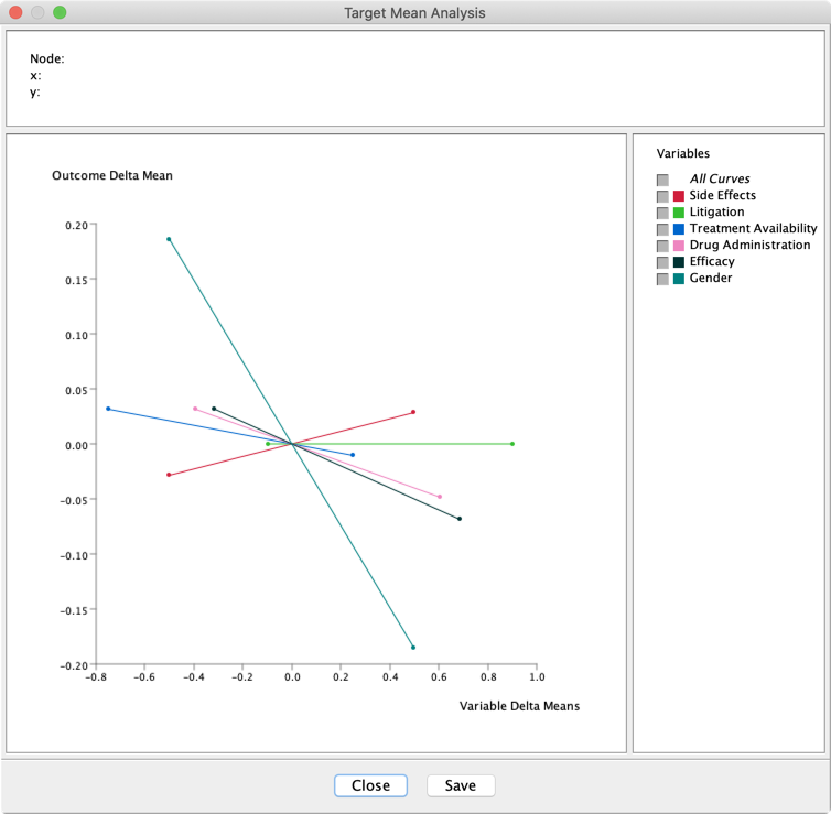
We can plot these curves with Main Menu > Analysis > Visual > Target > Target's Posterior > Curves > Total Effects.
For generating this graph, we can set a number of options:
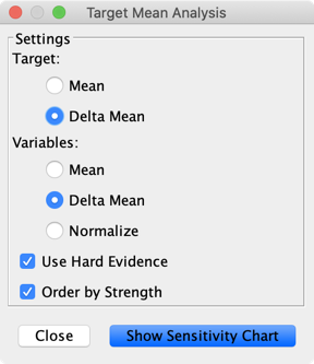
The x-axis, Variable Delta Means, represents the difference between the Mean Value generated for the analysis (here, Hard Evidence/Intervention on the states of the variable under study) and its Prior Mean Value. The y-axis represents the difference between the PosteriorMean Value of Outcome and its PriorMean Value.
If we do not specifically associate numerical values with symbolic states, BayesiaLab uses the state index. In our example,
- False is 0, and True is 1.
- Male is 0, and Female is 1.
- Not Recovered is 0, and Recovered is 1.
We see that Side Effects is the only variable with a positive causal effect. We also notice that Litigation has no causal effect.
Given that all variables are binary, the corresponding curves are linear. Therefore, the curves’ derivatives will be perfect summaries of the Total Effect Curves: Menu > Analysis > Report > Target > Total Effects on Target:
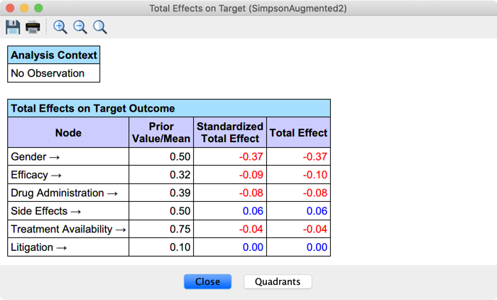
The Total Effect is the derivative computed at (0, 0) in the previous Target Mean Analysis graph, i.e., the slope of the curve. The Standardized Total Effect is the Total Effect times the ratio between the standard deviation of the variable and the standard deviation of the Target Node.
The arrow symbols (→) in the results table indicate that Intervention Mode was active on all nodes, triggering Graph Surgery upon each observation/intervention during the estimation of the effects.
Gender is the variable with the strongest Total Effect. It is negative because of the index values of the states. Females (1) are recovering at a lower rate than Males (0).
Note that there are two paths from Gender to Outcome (paths #1 and #2 illustrated in the previous section), and they are both causal. Gender is indeed a root node, i.e., it has no parents, meaning the Adjustment Criterion is fulfilled by default.
The Total Effect measures the effects of these two causal paths: the direct path (#1) and the indirect path (#2), represented by the dashed blue arcs below.
Direct Effects
Now suppose we are interested in estimating the effect of the direct paths only. This would require blocking not only the non-causal paths but also the indirect causal paths. This is the role of BayesiaLab’s Direct Effect functions. The only difference between Direct and Total Effect functions is that, by default, all other nodes are held constant during the estimation of the variable’s Direct Effect.
We generate the Direct Effect Curves with Menu > Analysis > Visual > Target > Target's Posterior > Curves > Direct Effects, using the same parameters as those previously used for Total Effects:
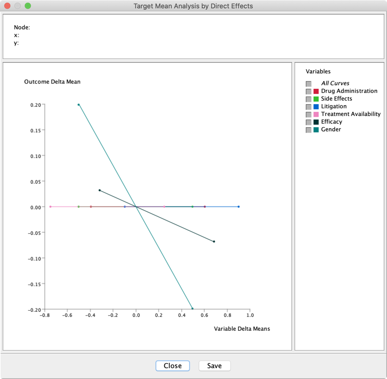
Given that all nodes are in Intervention Mode, the only variables with Direct Effects are the Parents of Outcome. Indeed, intervening on all nodes to hold them constant triggers Graph Surgery and generates the mutilated graph below:
The function Menu > Analysis > Report > Target > Direct Effects on Target allows us to compute the Direct Effects, the single-point estimates of these curves:
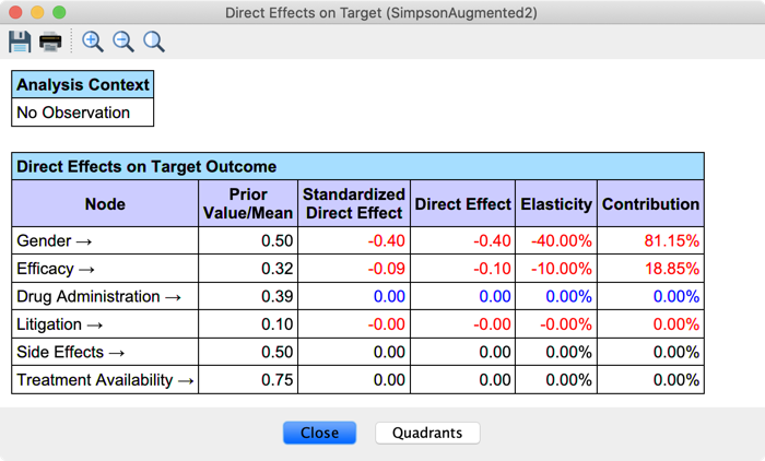
- The Direct Effect is the slope of the Direct Effect Curve between the endpoints of the variable interval.
- The Standardized Direct Effect is the Direct Effect times the ratio between the standard deviation of the variables and the standard deviation of the Target Node.
- The Elasticity is the Direct Effect times the ratio between the range of the variable and the range of the Target Node.
- The Contribution is the Standardized Direct Effect divided by the total sum of Standardized Direct Effects.
Non-Confounders
By default, BayesiaLab’s Direct Effect functions measure a variable’s effect by holding all other variables constant. However, we can use the predefined class Non_Confounder to define the nodes we do not want to control.
In our example, the main variable of interest, Drug Administration, has no direct effect. The post-treatment variable Efficacy mediates its causal effect, and the Direct Effect analysis blocks the path. We must therefore use the predefined class Non_Confounder (Efficacy’s Context Menu > Properties > Classes > Add > Predefined Class > Non_Confounders) to prevent BayesiaLab from holding Efficacy constant and allow the estimation of the mediated causal effect. The new mutilated graph below is then used for estimating the Direct Effects:
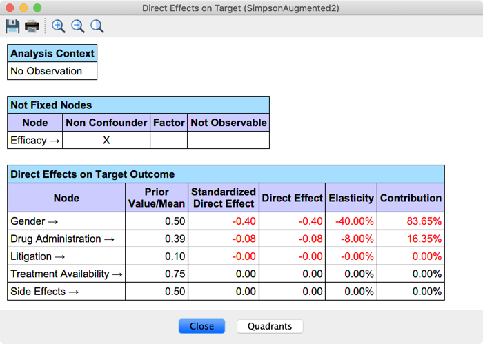
Drug Administration’s Direct Effect now equals the Average Causal Effect we manually computed with the Monitors. You can also note that we no longer analyze the effect of the Non-Confounder Efficacy.
Likelihood Matching
Now suppose we want to use Likelihood Matching instead of Graph Surgery. We first set back all nodes in Observation Mode via the monitors’ Contextual Menus.
Nodes of Interest: Treatments/Drivers
The nodes of interest are the nodes for which we want to estimate the causal effect on the Target Node. We call them Treatments or Drivers.
In the previous section, we assumed that all nodes were of interest and set them in Intervention Mode. With Likelihood Matching, the workflow is less straightforward. For each Driver, we need to analyze the paths to the Target (cf. Path Analysis) to define the set of nodes that need to be controlled for to block the non-causal paths and let the causal paths open. Note that these nodes’ sets may differ for each Driver, requiring us to perform multiple Total Effect analyses to avoid conflicting adjustments. The first step is then to define our nodes of interest. In the Augmented Simpson Paradox, the main variable of interest is obviously Drug Administration, but for illustrative purposes, let us consider Gender as well.
Total Effects
We have seen in the Path Analysis section that there are two paths between Gender and Outcome, both causal (#1 and #2). Thus, there is no variable to adjust for to estimate the Total Effect.
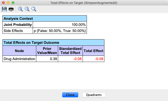
The Path Analysis indicates that there are also two paths between Drug Administration and Outcome, one causal (#7) and one non-causal (#6): Drug Administration ← Side Effects ← Gender → Outcome. So we need to adjust for Side Effects, or for Gender, to block this path. This is in contradiction to the analysis of Gender’s effect. We cannot estimate the Total Effects of Gender and Drug Administration in the same analysis with Likelihood Matching!
So let us start with Gender. We select the node, go to Menu > Analysis > Report > Target > Total Effects on Target, and confirm that we want to perform the analysis on the selected node only:
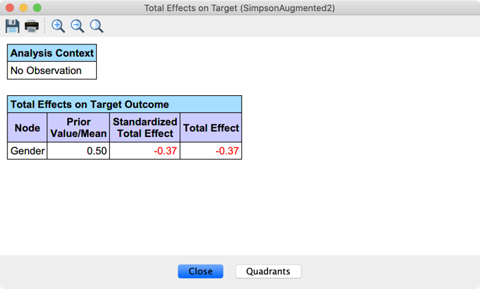
For Drug Administration, let us suppose we choose to adjust for Side Effects. We right-click on its associated Monitor and select Fix Probabilities from its Contextual Menu.
Then, we select the node Drug Administration, go to Analysis > Report > Target > Total Effects on Target, and confirm that we want to perform the analysis on the selected node only:
Direct Effects
Now let us look at the workflow for estimating Direct Effects with Likelihood Matching, i.e., how to assess the effects of the direct paths only. Remember that, by default, BayesiaLab’s Direct Effect functions measure a variable’s effect by holding all variables constant except those associated with the predefined class Non_Confounder. Holding a variable constant with Graph Surgery implies the deletion of its entering arcs. Thus, there is no risk of biasing the estimation of Direct Effects. In the Likelihood Matching case, this risk exists because we set evidence on the variable to adjust for it. Indeed, controlling for descendants of the Target Node (e.g., Litigation) automatically biases the estimate.
While we previously added Efficacy to the Non_Confounder class to let it mediate the effect of Drug Administration, we must also add Litigation to prevent its adjustment.
Notice that there is no conflict in this analysis:
- Gender
- Controlling for Side Effects, Drug Administration allows to cut the indirect causal path (#2);
- Controlling for Treatment Availability has no impact;
- Not controlling for Efficacy has no effect as path #2 is already blocked;
- Not controlling for Litigation prevents to bias the estimation of the effect;
- Drug Administration
- Controlling for Side Effects, Gender allows to cut the non-causal path (#4);
- Controlling for Treatment Availability has no impact;
- Not controlling for Efficacy allows to let the information flows from Drug Administration to Outcome;
- Not controlling for Litigation prevents to bias the estimation of the effect.
We can, therefore, select our two nodes of interest, use Analysis > Report > Target > Direct Effects on Target, and confirm that we want to perform the analysis on the selected nodes only:

Graph Surgery versus Likelihood Matching
Before concluding this chapter, let us summarize the main characteristics of Graph Surgery and Likelihood Matching:
- Graph Surgery
- requires a fully specified Causal Bayesian Network;
- uses the mutilated Causal Bayesian Network for causal inference;
- Likelihood Matching
- requires the causal analysis of the domain to define the variables that need to be adjusted for to block the non-causal paths and let the causal paths open;
- uses the Bayesian network to carry out probabilistic inference with the adjusted variables. Note that this network does not have to be causal! It just needs to represent the Joint Probability Distribution of the domain.
This last point is especially important. It is indeed sometimes challenging, if not impossible, to design the fully specified Causal Bayesian Network. However, BayesiaLab offers a wide range of machine-learning algorithms that we can use to induce a network that represents the Joint Probability Distribution. Hence, we only need to have a limited amount of causal knowledge to define the variables that have to be adjusted for.
For example, suppose we machine-learned the network below with Main Menu > Learning > Supervised Learning > Augmented Naive Bayes:
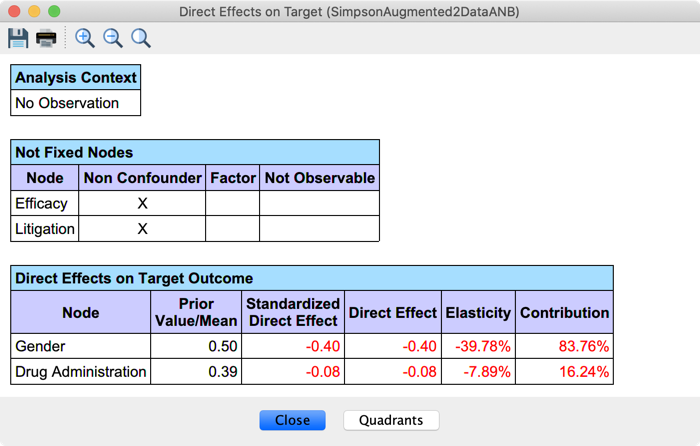
The main architecture of the network is Naïve, i.e., the Target Node is the parent of all nodes. Therefore, this Bayesian network is clearly not causal. If we were to use Graph Surgery, we would not find any total or direct effects (see the corresponding mutilated graph below when estimating the Direct Effects with Efficacy and Litigation defined as Non_Confounder).
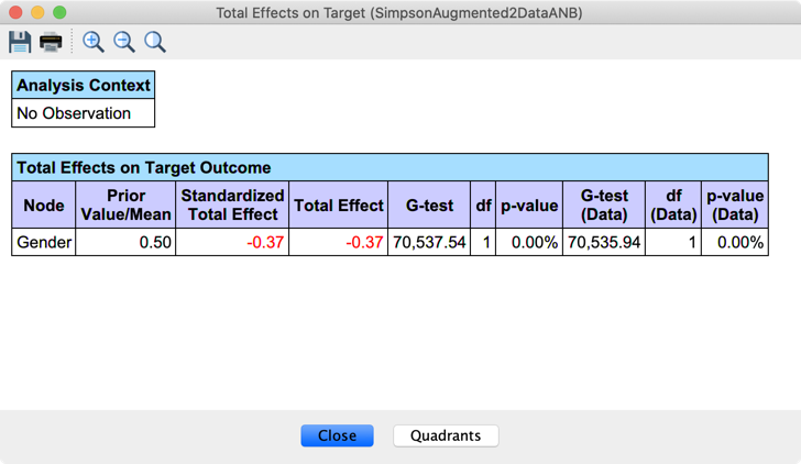
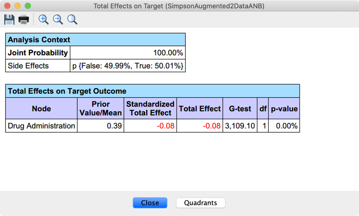
However, Likelihood Matching returns the correct estimations for the Total Effects with two separate analyses.
One analysis for Gender, without adjusting for any variables:
And one analysis for Drug Administration, by holding constant Side Effects:
As for Direct Effects, the analysis can be carried out for both variables with the current definition of Non_Confounders.
Conclusion
This chapter highlights how much effort is required to derive causal effect estimates from observational data. Simpson’s Paradox illustrates how much can go wrong even in simple circumstances. Given such potentially serious consequences, it is a must for policy analysts to examine all aspects of causality formally. To paraphrase Judea Pearl, we must not leave causal considerations to the mercy of intuition and good judgment. Fortunately, causality has emerged from its pariah status in recent decades, which has allowed tremendous progress in theoretical research and practical tools: “[…] practical problems relying on causal information that long were regarded as either metaphysical or unmanageable can now be solved using elementary mathematics” (Pearl, 1999).
