Means and Values of Nodes

Context

At the top of each Monitor, the items Mean, Dev, and Value are displayed.

Mean refers to the Mean Value m and is only shown in the Monitors of numerical nodes.

Dev stands for Standard Deviation and is shown alongside Mean.

Value refers to the Expected Value $v$ and is shown in all Monitors, regardless of the node type, i.e., categorical or numerical.

Examples

The calculations for Expected Value and Mean Value are shown in the context of the following examples:

Categorical Node

Let’s take the Discrete Nodes and Continuous Nodes Age with three categorical Node States:

• Child
• Adult
• Senior

Categorial Node with Assigned State Values

In the Node Editor, you can assign State Values to the Node States of Age.

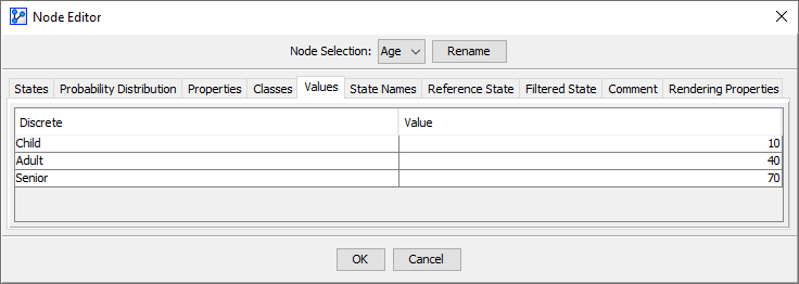
For each node, the Expected Value $v$ is computed using the assigned State Values and the marginal probability distribution of the Node States:

where $p$ is the marginal probability of state $s$ and $V_s$ is its associated value.

$v = 0.23 \times 10 + 0.415 \times 40 + 0.355 \times 70 = 43.750$

The Monitor shows $v$ as the Value of Age.

Discrete Numerical Variable

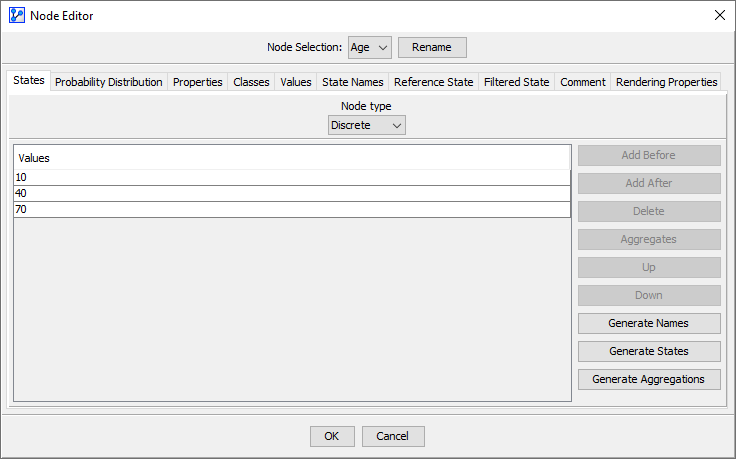
Let’s suppose that the node Age has three numerical Node States instead of categorical Node States.\

In this context, we need to consider two conditions, with and without State Values specified in the Node Editor:

No State Values Specified

Here, State Values are not specified in the Values tab of the Node Editor. Note the empty Value column below.

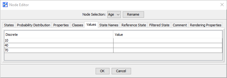
As a result, BayesiaLab uses the numerical values of the Node States, as they appear in the States tab, as the State Values.

Furthermore, as Age is a numerical node, its Monitor will now display the Mean (Mean) and the Standard Deviation (Dev) in addition to the Expected Value (Value)

The Mean m is computed using the numerical values of the Node States and the marginal probability distribution of the Node States:

where $c_s$ is the numerical value of the Node State.

$m = 0.23 \times 10 + 0.415 \times 40 + 0.355 \times 70 = 43.750$

State Values Specified

However, if State Values are separately specified in the Values tab of the Node Editor, they will be used for the calculation of Value in the Monitor.

To highlight the distinction between the Node States ${10, 40, 70}$ and the State Values, we assign unrelated arbitrary State Values of 0, 1, and 2.

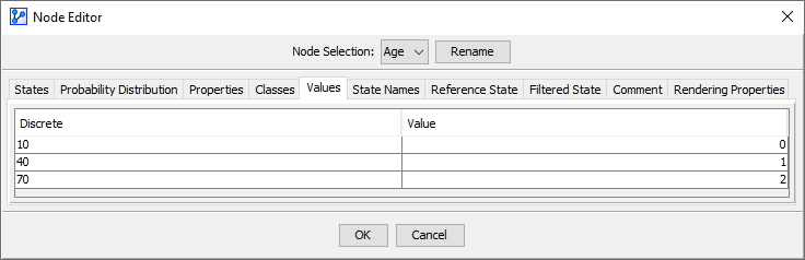
The Expected Value $v$ is computed now using the assigned State Values ${0, 1, 2}$ and the marginal probability distribution of the Node States:

where $p$ is the marginal probability of state $s$ and $V_s$ is its associated value.

$v = 0.23 \times 0 + 0.415 \times 1 + 0.355 \times 2 = 1.125$

The Monitor shows $v$ as the Value of Age.

Continuous Numerical Variable

Let’s now consider a continuous variable Age defined in the domain [0; 99], discretized into three states:

• Child: [0 ; 18]
• Adult: ]18 ; 65]
• Senior: ]65 ; 99]

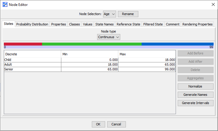
Given that Age is a numerical node, its Monitor shows the Mean (Mean), the Standard Deviation (Dev), plus the Expected Value (Value).

No Associated Data

If no associated data is with the node, both $c_s$ and $V_s$ are defined as the mid-points of the minimum and maximum values of each Node State. For example, for the Node State Adult ]18; 65], the midpoint is 17.2225.

So, the Mean Value m is computed as follows:

$m = 0.23 \times 9 + 0.415 \times 41.5 + 0.355 \times 82 = 48.4025$

The Expected Value $v$ is calculated analogously:

$v = 0.23 \times 9 + 0.415 \times 41.5 + 0.355 \times 82 = 48.4025$\

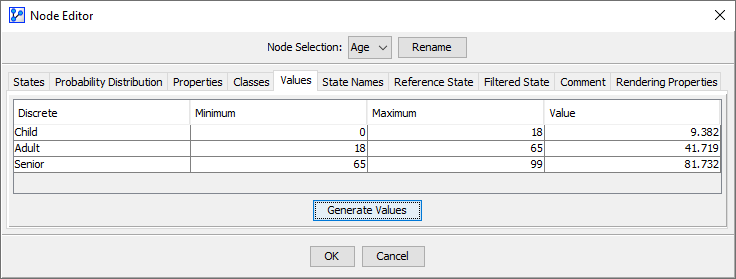
Associated Data

If data is associated with the node, $c_s$ is defined as the arithmetic mean of the data points that are associated with each Node State.

Furthermore, clicking on the Generate Values button in the Node Editor sets the values $Vs$ to the current arithmetic means of each Node State.

Value Delta

If you set a new piece of evidence on a node that modifies the distribution of the node, the Monitor displays a delta value in parentheses adjacent to Value.

This delta is the difference between the current Expected Value $v$ and:

• the Expected Value $v$ before setting the modifying evidence, or
• the Expected Value $v$ that corresponds to the Reference Probability Distribution, which you can set with the icon in the toolbar.

Special Case: Some Node States Without Values

If only some Node States have an associated value, the Expected Value $v$ is computed from the subset of Node States $S^*$ that do have an associated value.

If a node only has a single Node State with an associated value, the corresponding Monitor does not report the Expected Value $v$.