Inference
Inference
Throughout this book so far, we have performed inference with various types of evidence. The nature of the problem domain routinely determined the kind of evidence we used.
We will now use this example to systematically try out all types of evidence for performing inference. With that, we depart from our habit of showing only realistic applications. One could certainly argue that not all types of evidence are plausible in the context of a Bayesian network that represents the stock market. In particular, any inference we perform here with arbitrary evidence should not be interpreted as an attempt to predict stock prices. Nevertheless, for the sake of an exhaustive presentation, even this somewhat contrived exercise shall be educational.
Within our large network of 459 nodes, we will only focus on a small subset of nodes, namely PG (Procter & Gamble), JNJ (Johnson & Johnson), and KMB (Kimberly-Clark). These nodes come from the “neighborhood” shown earlier.
We highlight PG, JNJ, and KMB to bring up their Monitors. Prior to setting any evidence, we see their marginal distributions in the Monitors. We see that the expected value (mean value) of the returns is 0.

Inference with Hard Evidence
Next, we double-click the state JNJ>0.012 to compute the posterior probabilities of PG and KMB, given this evidence. The gray arrows indicate how the distributions have changed compared to before, prior to setting evidence. Given the evidence, the expected values of PG and KMB are now 1.2% and 0.6%, respectively.

If we also set KMB to its highest state (KMB>0.012), this would further reduce the uncertainty of PG and compute an expected value of 1.8%. This means that PG had an average daily return of 1.8% on days when this evidence was observed.

Inference with Probabilistic and Numerical Evidence
Given the discrete states of nodes, setting Hard Evidence is presumably intuitive to understand. However, the nature of many real-world observations calls for so-called Probabilistic Evidence or Numerical Evidence. For instance, the observations we make in a domain can include uncertainty. Also, Evidence Scenarios can consist of values that do not coincide with the values of nodes’ states. So, as an alternative to Hard Evidence, we can use BayesiaLab to set such evidence.
Probabilistic Evidence
Probabilistic Evidence is a convenient way of directly encoding our assumptions about possible conditions of a domain. For example, a stock market analyst may consider a scenario with a specific probability distribution for JNJ corresponding to a hypothetical period of time (i.e., a subset of days). Given his understanding of the domain, he can assign probabilities to each state, thus encoding his belief.
After removing the prior evidence, we can set such beliefs as Probabilistic Evidence by right-clicking the JNJ Monitor and then selecting Enter Probabilities.
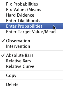
For the distribution of Probabilistic Evidence, the sum of the probabilities must be equal to 100%. We can adjust the Monitor’s bar chart by dragging the bars to the probability levels that reflect the scenario under consideration. By double-clicking on the percentages, we can also directly enter the desired probabilities. Note that changing the probability of any state automatically updates the probabilities of all other states to maintain the sum constraint.
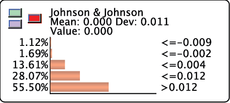
To remove a degree of freedom in the sum constraint, we left-click the State Name/Value in the Monitor to the right of each bar. Doing so locks the currently set probability and turns the corresponding bar green. The probability of this state will no longer be automatically updated while the probabilities of other states are being edited. This feature is essential for defining a distribution on nodes with more than two states. Another left-click on the same State Name/Value unlocks the probability again.
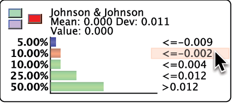
There are two ways to validate the entered distribution, via the green and the purple buttons. Clicking the green button defines a static likelihood distribution. This means that any additional piece of evidence on other nodes can update the distribution we set.
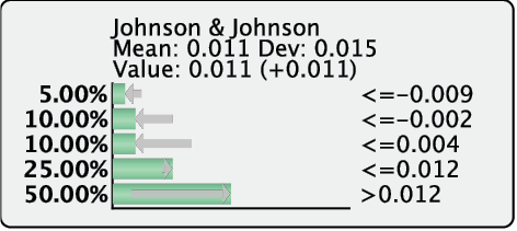
Clicking the purple button “fixes” the probability distribution we entered by defining dynamic likelihoods. This means that each new piece of evidence triggers an update of the likelihood distribution in order to maintain the same probability distribution.
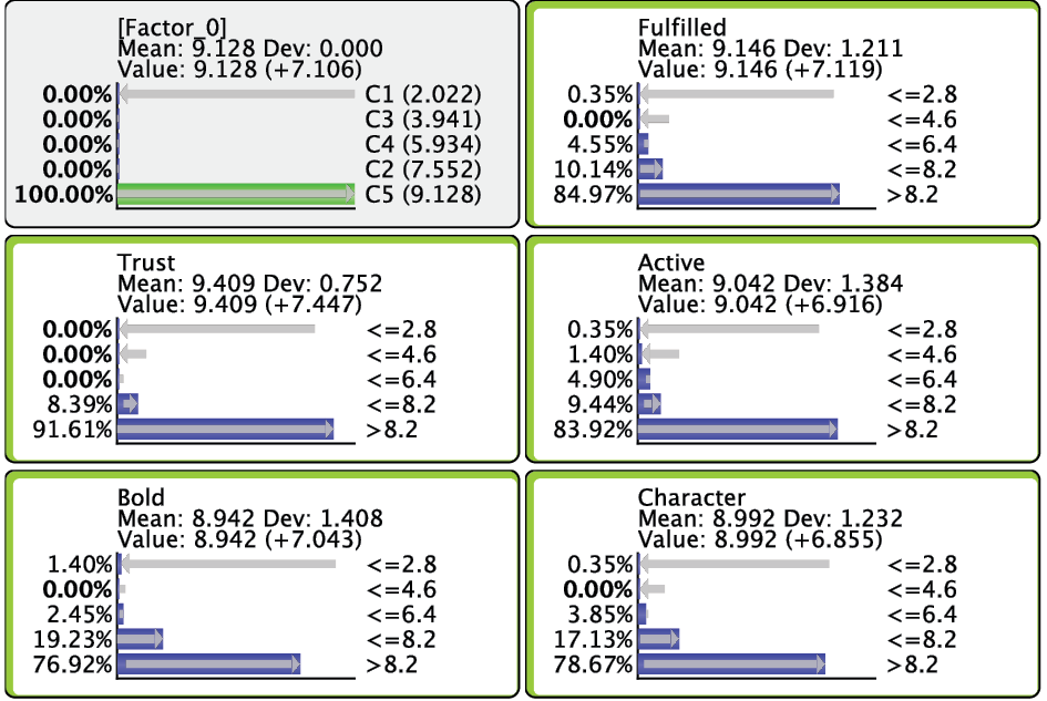
Using either validation method, BayesiaLab computes a likelihood distribution that produces the requested probability distribution. By setting this distribution, BayesiaLab also performs inference automatically and updates the probabilities of the other nodes in the network.

Numerical Evidence
Instead of a specific probability distribution, an observation or scenario may exist as a single numerical value, meaning we must set Numerical Evidence. For instance, a stock market analyst may wish to examine how other stocks performed given a hypothetical period of time during which the average of the daily returns of JNJ was −1%. Naturally, this requires that we set evidence on JNJ with an expected (mean) value of −0.01 (=−1%). However, this task is not as straightforward as it may sound. The question will become apparent as we follow the steps to set this evidence.
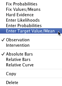
First, we right-click JNJ Monitor and then select Enter Target Value/Mean from the Contextual Menu.
Next, we type “−0.01” into the dialog box for Target Mean/Value. Additionally, as was the case with Probabilistic Evidence, we have to choose the type of validation, but we now have three options under Observation Type:
- No Fixing, which is the same as the green button , i.e., validation with static likelihood.
- Fix Mean, which is the same as the purple button, except that the likelihood is dynamically computed to maintain the mean value, although the probability distribution can change as a result of setting additional evidence.
- Fix Probabilities, which is the same as the purple button , i.e., validation with dynamic likelihood.
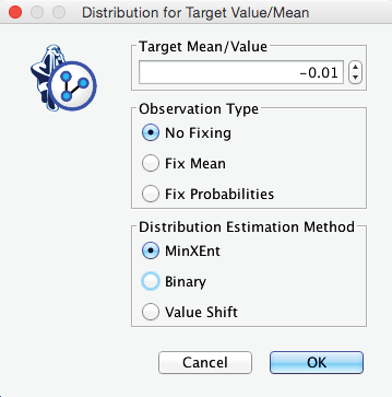
Apart from setting the validation method, we also need to choose the Distribution Estimation Method, as we need to come up with a distribution that produces the desired mean value. Needless to say, there is a great number of distributions that could potentially produce a mean value of −0.01. However, which one is appropriate?
To make a prudent choice, we must first understand what the evidence represents. Only then can we choose from the three available algorithms for generating the Target Distribution that will produce the Target Mean/Value.
MinXEnt (“Minimum Cross-Entropy”)
Using the MinXEnt algorithm, the Target Distribution, which produces the Target Mean/Value, is computed so that the Cross-Entropy between the original probability distribution of the node and the Target Distribution is minimized. The Monitor below shows the distribution with a mean of −0.01, which is “closest” in terms of Cross-Entropy to the original marginal distribution shown earlier.

Binary
If we select Binary, the Target Mean/Value is generated by interpolating between values of two adjacent states, hence the name. Here, a “mix” of the values of two states, i.e., JNJ <=−0.009 and JNJ <=−0.002, produces the desired mean of −0.01.

Value Shift
With Value Shift, the Target Mean/Value is generated by shifting the values of each particle (or virtual observation) by the exact same amount.

Target Value/Mean Considerations
As we see in the examples above, using different Target Distributions as Numerical Evidence—albeit with the same mean value—results in different probability distributions.
Binary
The Binary algorithm produces the desired value through interpolation, as in Fuzzy Logic. Among the three available methods, it generates distributions that have the lowest degree of uncertainty. Using the Binary algorithm for generating a Target Mean/Value would be appropriate if two conditions are met:
- There is no uncertainty regarding the evidence, i.e., we want the evidence to represent a specific numerical value. “No uncertainty” would typically apply in situations in which we want to simulate the effects of nodes that represent variables under our control.
- The desired numerical value is not directly available by setting Hard Evidence. In fact, a distribution produced by the Binary algorithm would coincide with Hard Evidence if the requested Target Value/Mean precisely matched the value of a particular state.
Given that it is impossible to set prices in the stock market directly, it is clearly not a good example for illustrating this using the Binary algorithm. Perhaps a price elasticity model would be more appropriate. In such a model, we would want to infer sales volume based on one specific price level instead of a broad range of price levels within a distribution.
MinXEnt and Value Shift
The other two algorithms, MinXEnt and Value Shift, generate Soft Evidence. This means that the Target Distribution they supply should be understood as posterior distribution given evidence set on a “hidden cause”, i.e., evidence on a variable not included in the model. As such, using MinXEnt or Value Shift is suitable for creating evidence that represents changing levels of measures like customer satisfaction. Unlike setting the price of a product, we cannot directly adjust the satisfaction of all customers to a specific level. This would imply setting an unrealistic distribution with low or no uncertainty.
More realistically, we would have to assume that higher satisfaction results from an enhanced product or better service, i.e., a cause from outside the model. Thus, we need to generate evidence for customer satisfaction as if a hidden cause produced it. This also means that MinXEnt and Value Shift will produce a distribution close to the marginal one if the targeted Numerical Evidence is close to the marginal value.
Special Cases of Numerical Evidence
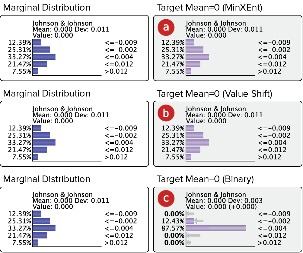
If the Numerical Evidence equals the current expected value, using MinXEnt (a) or Value Shift(b) will not change the distribution. Using the Binary algorithm (c), however, will return a different distribution (except in the context of a binary node).
Conflicting Evidence
In the examples shown so far, setting evidence typically reduced uncertainty with regard to the node of interest. Just by visually inspecting the distributions, we can tell that setting evidence generally produces “narrower” posterior probabilities.
However, this is not always the case. Occasionally, separate pieces of evidence can conflict with each other. We illustrate this by setting such evidence on JNJ and KMB. We start with the marginal distribution of all nodes.

After setting Numerical Evidence (using MinXEnt) with a Target Mean/Value of +1.5% on JNJ.

The posterior probabilities inferred from the JNJ evidence indicate that the PG distribution is more positive than before. More importantly, the uncertainty regarding PG is lower. A stock market analyst would perhaps interpret the JNJ movement as a positive signal and hypothesize about a positive trend in the CPG industry. In an effort to confirm his hypothesis, he would probably look for additional signals that either confirm the trend and the related expectations regarding PG and similar companies.
In the KMB Monitor, the gray arrows and “(+0.004)” indicate that the first evidence increases the expectation that KMB will also increase in value. If we observed, however, that KMB decreased by 1.5% (once again using MinXEnt), this would go against our expectations.

The result is that we now have a more uniform probability distribution for PG—rather than a narrower distribution. This increases our uncertainty about the state of PG compared to the marginal distribution.
Even though it appears that we have “lost” information by setting these two pieces of evidence, we may have a knowledge gain after all: we can interpret the uncertainty regarding PG as a higher expectation of volatility.
Measures of Conflict
Beyond a qualitative interpretation of contradictory evidence, our Bayesian network model allows us to examine “conflict” beyond its common-sense meaning. A formal conflict measure can be defined by comparing the joint probabilities of the current model versus a reference model, given the same set of evidence for both.
A fully unconnected network is commonly used as the reference model, the so-called “straw model.” It is a model that considers all nodes to be marginally independent. If the joint probability of the set of evidence returned by the model under study is lower than that of the reference model, we determine that we have a conflict. Otherwise, if the joint probability is higher, we conclude that the pieces of evidence are consistent.
The conflict measures that are available in BayesiaLab are formally defined as follows:
Global Conflict (Overall Conflict)
where is the current set of evidence consisting of observations and is the piece of evidence.
Bayes Factor
where is a hypothetical piece of evidence that has not yet been set or observed.
Local Conflict (Local Consistency)
Evidence Analysis Report
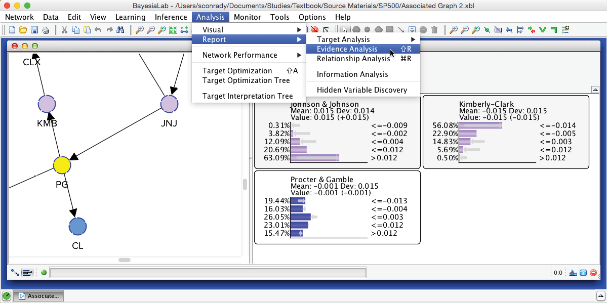
Using these definitions, we can compute to what extent a new observation would be consistent with the current set of evidence. BayesiaLab provides us with this capability in the form of the Evidence Analysis Report, which can be generated by selecting Menu > Analysis > Report > Evidence Analysis from the main menu.
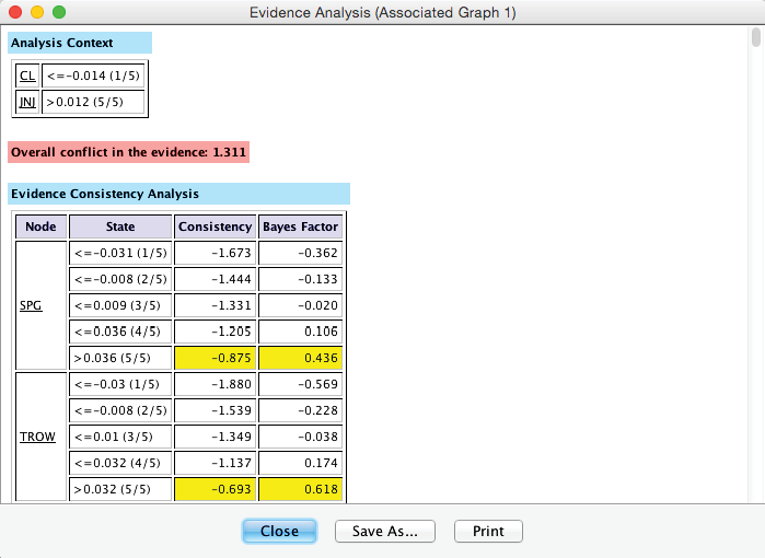
The Evidence Analysis Report displays two closely-related metrics, Local Consistency (LC) and the Bayes Factor (BF), for each state of each unobserved node in the network, given the set of evidence. The top portion of this report is shown below. Also, as we anticipated, an Overall Conflict between the two pieces of evidence is shown at the top of the report.
Summary
Unsupervised Learning is a practical approach for obtaining a general understanding of simultaneous relationships between many variables in a database. The learned Bayesian network facilitates visual interpretation plus the computation of omnidirectional inference, which can be based on any type of evidence, including uncertain and conflicting observations. Given these properties, Unsupervised Learning with Bayesian networks becomes a universal tool for knowledge discovery in high-dimensional domains.
