Product Optimization
In order to perform optimization for a particular product, we need to open the network for that specific product. Networks for all products were automatically generated and saved during the Multi-Quadrant Analysis, so we need to open the network for the product of interest. The suffix in the file name reflects the Product.
.png)
To demonstrate the optimization process, we open the file that corresponds to Product 1. Structurally, this network is identical to the network learned from the entire dataset. However, the parameters of this network were estimated only on the basis of the observations associated with Product 1.
.png)
Now we have all the elements that are necessary for optimizing the Purchase Intent of Product 1:
- A network that is specific to Product 1;
- A set of driver variables, selected by excluding the non-driver variables via Costs;
- Realistic scenarios, as determined by the Variation Domains of each driver variable.
With the above, we are now able to search for node values that optimize Purchase Intent.
Target Dynamic Profile
Before we proceed, we need to explain what we mean by optimization. As all observations in this study are consumer perceptions, it is clear that we cannot directly manipulate them. Rather, this optimization aims to identify in which order the perfume maker should address these perceptions. Some consumer perceptions may relate to specific odoriferous compounds that a perfumer can modify; other perceptions may be influenced by marketing and branding initiatives. However, the precise mechanism of influencing consumer perceptions is not the subject of our discussion. From our perspective, the causes that could influence the perception are hidden. Thus, we have here a prototypical application of Soft Evidence, i.e., we assume that the simulated changes in the distribution of consumer perceptions originate in hidden causes (see Numerical Evidence in Chapter 7).
While BayesiaLab offers a number of optimization methods, Target Dynamic Profile is appropriate here. We start it from within Validation Mode F5 by selecting Menu > Analysis > Report > Target Analysis > Target Dynamic Profile.
.png)
We need to explain the many options that must be set for Target Dynamic Profile. These options will reflect our objective of pursuing realistic sets of evidence:
.png)
In Profile Search Criterion, we specify that we want to optimize the mean value of the Target Node as opposed to any particular state or the difference between states.
Joint Probability
Next, we specify under Criterion Optimization that the mean value of the Target Node is to be maximized. Furthermore, we check Take Into Account the Joint Probability. This weights any potential improvement in the mean value of the Target Node by the joint probability corresponding to the set of simulated evidence that generated this improvement. The joint probability of a simulated Evidence Scenario will be high if its probability distribution is close to the original probability distribution observed in the consumer population: the higher the joint probability, the closer the simulated scenario to the status quo of customer perception.
In practice, checking this option means that we prefer smaller improvements with a high joint probability over larger ones with a low joint probability: 0.146 × 26.9% = 0.0393 > 0.174 × 21.33% = 0.0371.
.png)
If all simulated values were within the constraints set in the Variation Editor, it would be better to increase the driver variable Spiced to a simulated value of 7 rather than 7.5, even though Purchase Intent would be higher for the latter value of Spiced. In other words, the “support” for E(Spiced)=7 is greater than for E(Spiced)=7.5, as more respondents are already in agreement with such a scenario. Once again, this is about pursuing achievable improvements rather than proposing pie-in-the-sky scenarios.
Costs
In this example, so far, we have only used Costs for selecting the subset of driver variables. Additionally, we can utilize Costs in the original sense of the word in the optimization process. For instance, if we had information on the typical cost of improving a specific rating by one unit, we could enter such a value as cost. This could be a dollar value, or we could set the costs to reflect the relative effort required for the same amount of change, e.g., one unit, in each driver variable. For example, a marketing manager may know that it requires twice as much effort to change the perception of Feminine compared to changing the perception of Sweet. If we want to quantify such efforts by using Costs, we must ensure that all variables’ costs share the same scale. For instance, if some drivers are measured in dollars and others are measured in terms of time spent in hours, we will need to convert hours to dollars.
In our study, we leave all the included driver variables at a Cost of 1, i.e., we assume that it requires the same effort for the same amount of change in any driver variable. Hence, we can leave the Utilize Evidence Cost unchecked (Not Observable nodes still remain excluded as driver variables).
Compute Only Prior Variations needs to remain unchecked as well. This option would be useful if we were interested in only computing the marginal effect of drivers. We would not want any cumulative effects or conditional variations given other drivers for that purpose.
Associate Evidence Scenario will save the identified sets of evidence for subsequent evaluation.
The setting of Search Methods is critically important for the optimization task. We need to define how to search for sets of evidence. Using Hard Evidence means that we would exclusively try out sets of evidence consisting of nodes with one state set to 100%. This would imply that we simulate a condition in which all consumers perfectly agree with regard to some ratings. Needless to say, this would be utterly unrealistic. Instead, we will explore sets of evidence consisting of distributions for each node by modifying their mean values as Soft Evidence. More precisely, we use the MinXEnt method to generate such evidence (see Minimum Cross-Entropy in Chapter 7).
In this context, we reintroduce the Variations we saved earlier. We reason that the best-rated product with regard to a particular attribute represents a plausible upper limit for what any product could strive for in terms of improvement. This also means that a driver variable that has already achieved the best level will not be optimized further in this framework.
Variation Editor
Clicking on Variations brings up the Variation Editor. By default, it shows variations in the amount of ±100% of the current mean.
.png)
To load the Variations we generated earlier through Multi-Quadrant Analysis, we click Import and select Absolute Variations from the pop-up window.
.png)
Now, we can open the previously saved file.
.png)
The Variation Editor now reflects the constraints. Any available expert knowledge can be applied here by entering new values for the Minimum Mean or Maximum Mean or by entering percent values for Positive Variations and Negative Variations.
Depending on the setting, the percentages are relative to (a) the Mean, (b) the Domain, or (c) the Progression Margin.
.png)
Selecting the Progression Margin is particularly useful as it automatically constrains the positive and negative variations in proportion to the gap from the Current Mean to the Maximum Mean and Minimum Mean values, respectively. In other words, it limits the improvement potential of a driver variable as its value approaches the maximum. It is a practical—albeit arbitrary—approach to prevent overly optimistic optimizations.
.png)
Next, we select MinXEnt in the Search Method panel as the method for generating Soft Evidence. In terms of Intermediate Points, we set a value of 20. This means that BayesiaLab will simulate 22 values for each node, i.e., the minimum and maximum plus 20 intermediate values, all within the constraints set by the variations. This is particularly useful in the presence of non-linear effects.
Within the Search Stop Criteria panel, the Maximum Size of Evidence specifies the maximum number of driver variables recommended as part of the optimization policy. Real-world considerations once again drive this setting. Although one could wish to bring all variables to their ideal level, a decision-maker may recognize that it is not plausible to pursue anything beyond the top 4 variables.
Alternatively, we can choose to terminate the optimization process once the joint probability of the simulated evidence drops below the specified Minimum Joint Probability.
The final option, Use the Automatic Stop Criterion, leaves it up BayesiaLab to determine whether adding further evidence provides a worthwhile improvement for the Target Node.
Optimization Results
Once the optimization process concludes, we obtain a report window that contains a list of priorities: Personality, Fruity, Flowery, and Tenacious.
.png)
To explain the items in the report, we present a simplified and annotated version of the report below. Note that this report can be saved in HTML format for subsequent editing as a spreadsheet.
Most importantly, the Value/Mean column shows the successive improvement upon implementing each policy. From initially 3.58, the Purchase Intent improves to 3.86, which may seem like a fairly small step. However, the importance lies in the fact that this improvement is not based on Utopian thinking but rather on modest changes in consumer perception, well within the range of competitive performance.
Evidence Scenarios
As an alternative to interpreting the static report, we can examine each element in the list of priorities. To do so, we bring up all the Monitors of the nodes identified for optimization.
.png)
Then, we retrieve the individual steps by right-clicking on the Evidence Scenario icon in the lower right-hand corner of the main window.
.png)
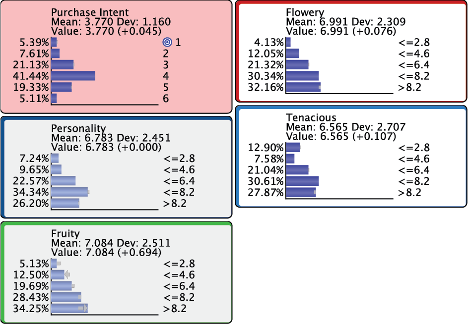
Selecting the first row in the table (Index=0) sets the evidence corresponding to the first priority, i.e., Personality. We can now see that the evidence we have set is a distribution rather than a single value. The small gray arrows indicate how the distribution of the evidence and the distributions of Purchase Intent, Fruity, Flowery, and Tenacious, are all different from their prior marginal distributions. The changes to the Fruity, Flowery, and Tenacious correspond to what is shown in the report in the column Value/Mean at T.
.png)
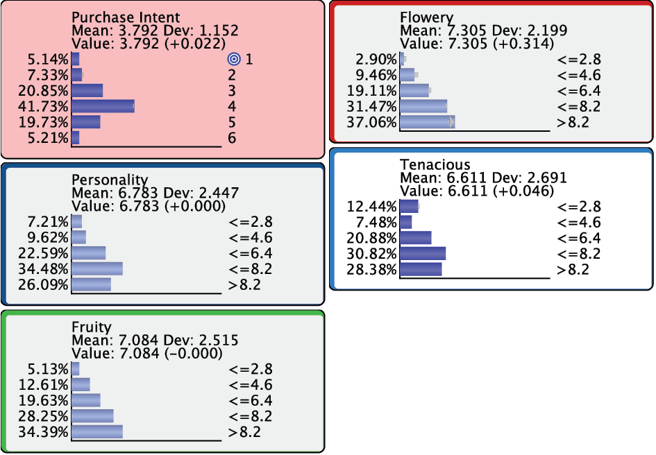
By selecting Index=1 we introduce a second set of evidence, i.e., the optimized distribution for Personality.

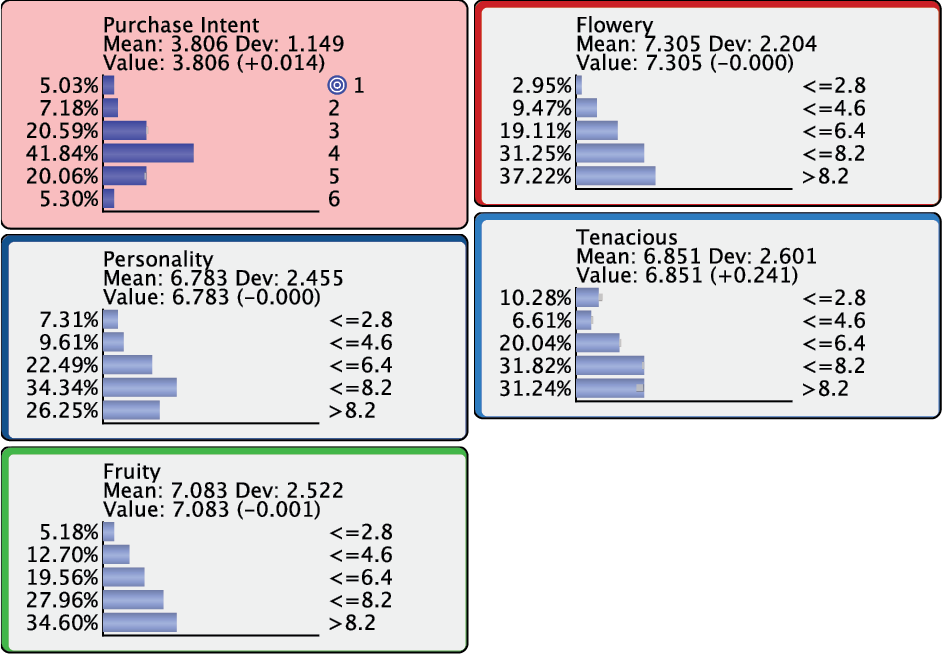
Continuing with Index 2 and 3, we see that the improvements to Purchase Intent become smaller.


Bringing up all the remaining nodes would bring up any “collateral” changes due to setting multiple pieces of evidence.
The results tell us that for Product 1, a higher consumer rating of Personality would be associated with a higher Purchase Intent. Improving the perception of Personality might be a task for the marketing and advertising team. Similarly, a better consumer rating of Fruity would also be associated with greater Purchase Intent. A product manager could then interpret this and request a change to some ingredients. Our model tells us that if such changes in consumer ratings were brought about in the proposed order, a higher Purchase Intent would potentially be observed.
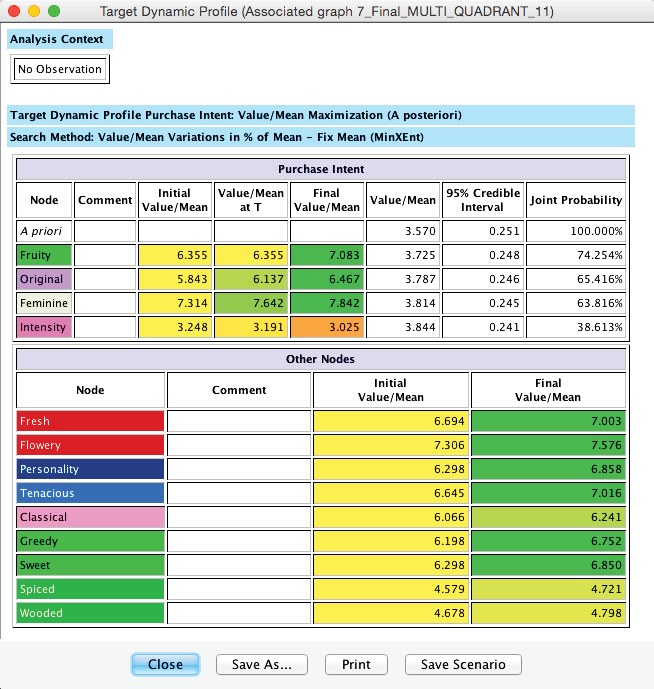
While we have only presented the results for Product 1, we want to highlight that the priorities are different for each product, even though they all share the same underlying PSEM structure. The recommendations from the Target Dynamic Profile of Product 11 are shown below.

This is an interesting example as it identifies that the JAR-type variable Intensity needs to be lowered to optimize Purchase Intent for Product 11.
It is important to reiterate that the sets of evidence we apply are not direct interventions in this domain. Hence, we are not performing causal inference. Instead, the sets of evidence we found help us prioritize our course of action for product and marketing initiatives.
Summary
We presented a complete workflow that generates a Probabilistic Structural Equation Model for key driver analysis and product optimization. The Bayesian networks paradigm turned out to be a practical platform for developing the model and its subsequent analysis all the way through optimization. With all the steps contained in BayesiaLab, we have a single, continuous line of reasoning from raw survey data to a final order of priorities for action.
