Confidence Intervals Analysis

Context

• The Confidence Intervals Analysis helps interpret a wide range of metrics relating to nodes in a Bayesian network.
• In many of BayesiaLab’s reports, such as the Target Analysis Report, quantities are displayed as single-point estimates, for instance, the mean value of a node, or the Mutual Information between two nodes.
• When comparing such values across several nodes, single-point estimates are not enough to judge which node is higher or more important.
• Importantly, we need to take into account the uncertainty associated with any estimates, regardless of whether the uncertainty comes from assessments or from a small sample size.
• Before we explain the workflow for the Confidence Intervals Analysis, we need to take a step back to recapitulate the Confidence Intervals Report.

Confidence Intervals Report

• To run the Confidence Intervals Report, go to Main Menu > Network > Reports > Confidence Intervals.

  • For BayesiaLab to construct the desired Confidence Intervals, you need to specify a Confidence Level in Preferences.

  • Go to Main Menu > Window > Preferences > Tools > Statistical Tools.

  • Select the desired value from the Confidence Level dropdown menu.

    

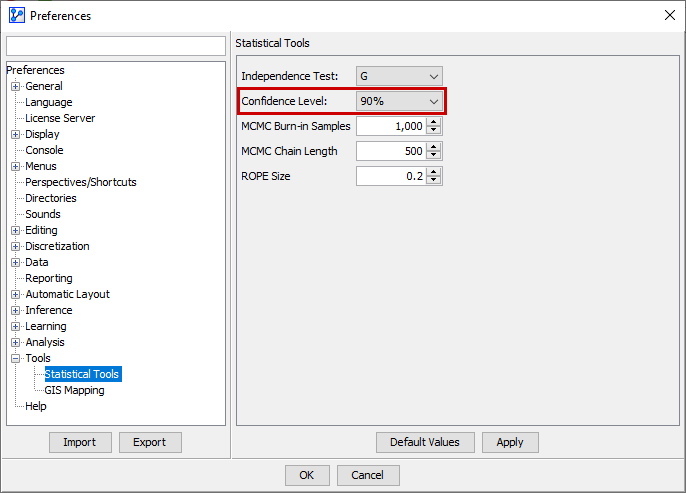
  • For example, if you specify a Confidence Level of 90%, it means that BayesiaLab constructs the Confidence Intervals so that there is a 90% probability that the true parameter value $\theta$ falls within the Confidence Intervals of the parameter estimate $\widehat{\theta}$.

  • Note that your selection of the Confidence Level also applies to all other statistical tools and tests used in BayesiaLab, including the Confidence Intervals Analysis explained below.

Confidence Intervals Analysis

• To start the Confidence Intervals Analysis, go to Main Menu > Analysis > Visual > Sensitivity > Confidence Intervals.
• The Confidence Intervals Analysis constructs the Confidence Intervals exactly the same way the Confidence Intervals Report described above.
• This process is conceptualized in the following diagram. It shows the probability densities of the parameter estimates.
  Loading SVG...

  Click to Zoom

Monte Carlo Simulation

• Next, BayesiaLab performs a Monte Carlo Simulation by sampling probabilities from the constructed Confidence Intervals and creating a Bayesian network for each sample.

• In this context, you need to specify the number of samples BayesiaLab draws from the parameter distributions for generating the corresponding Bayesian networks.

  

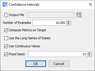
• Setting a value of 10,000 means that BayesiaLab will generate 10,000 Bayesian networks with parameters sampled from the Confidence Intervals.

• Then, these 10,000 networks are evaluated in terms of how the sampled parameters affect the Joint Probability Distribution.

• The Confidence Intervals Analysis Report calculates the following items:

  • States’ Probabilities
  • Mean

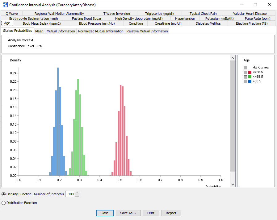
The screenshot shows the distributions of the State Probabilities of the node Age.

• Furthermore, if the network contains a Target Node, and you set the Compute Metrics on Target option, BayesiaLab also computes the following metrics for each node with regard to the Target Node.
  • Mutual Information
  • Normalized Mutual Information
  • Relative Mutual Information

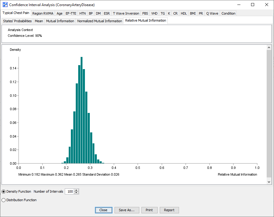
The following screenshot shows the distribution of Relative Mutual Information of the node Typical Chest Pain with regard to the Target Node Condition.

Workflow Illustration

• To demonstrate this workflow, we use the Coronary Artery Disease network, which you can download here:

  

  CoronaryArteryDisease.xbl

  XBL

• In this example, we run the Confidence Intervals Analysis on all nodes.

• Next, we select Relative Mutual Information as the metric of interest and sort the tabs accordingly.

• Each tab at the top of the window represents one node in the network.

• As we click through the tabs from left to right, we observe that the Relative Mutual Information decreases.

• This is in sync with what we would obtain from a Target Analysis Report: Main Menu > Analysis > Report > Target > Relationship with the Target Node.

• We show the corresponding report here just for reference:

  

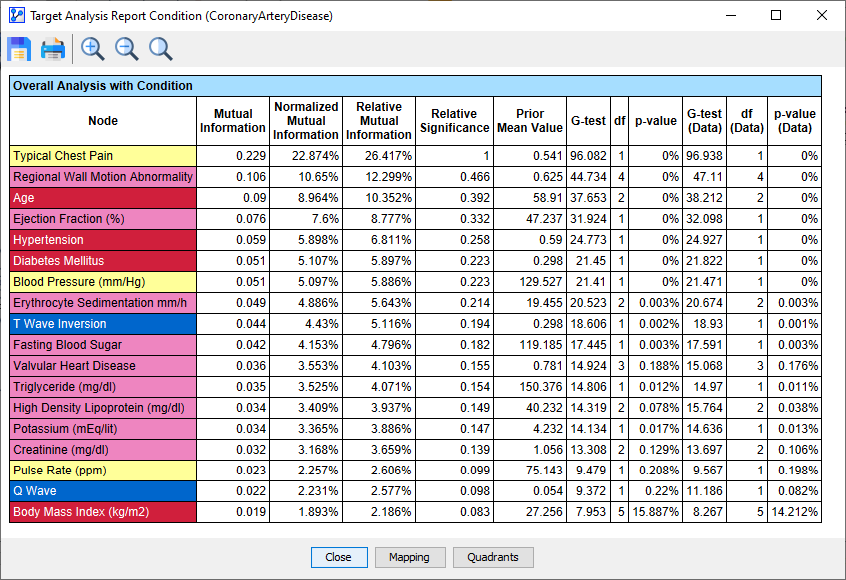
• We may now be tempted to read this report as a hierarchy in terms of importance.

• However, we need to be careful about such conclusions. The following animation highlights the issue:

• By overlaying the distributions of the Relative Mutual Information values, we can only find that Typical Chest Pain is clearly distinct from the remaining nodes.

• The Relative Mutual Information distributions of the remaining nodes seem to blend into each other, which implies that the hierarchy the Target Analysis Report above suggests isn’t nearly as clear.

• As a result, we need to be careful with any claims regarding a rank order of the nodes unless the Confidence Intervals Analysis demonstrates clearly separated distributions.