Consistency
Context
The Consistency (also called Conflict ) allows comparing two joint probabilities of an n-dimensional evidence :
- the joint probability of the reference model, i.e. the current Bayesian network that represents the dependencies between the variables,
- the joint probability of the straw model, i.e. the fully unconnected network, in which all the variables are marginally independent.
where and are the log-losses associated with the evidence by using the straw model () and the reference model () respectively.
The log-loss reflects the cost (in bits) per instance of using our model, i.e. the number of bits that are needed to encode the probability of the pieces of evidence. The lower the probability is, the higher the log-loss is.
The Consistency is positive if the joint probability computed with the reference model is higher than the one computed with the straw model. Conversely, a negative Consistency indicates a so-called Conflict, as the joint probability of the evidence is higher with the model with all independent variables compared to the model that includes dependencies.
Note that conflicting evidence does not necessarily mean that the reference model is wrong. Rather, it usually indicates that this evidence belongs to the tail of the distribution represented by the reference model. However, if the evidence is drawn from the reference model’s distribution, the probability of observing conflicting evidence should be less than the probability of observing consistent evidence. Thus, the mean of the consistencies has to be positive, otherwise, the reference model does not fit the joint probability distribution sampled by the evidence.
The strength of the dependencies that are represented in the reference model increases the difference between the probabilities of conflicting and consistent evidence, and the Consistency/Conflict values as well. The Consistency Mean is, therefore, a good way to measure the overall strength of a model.
Example
Let’s suppose we have the following reference structure with 2 boolean nodes, and :

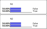
Four different sets of two-dimensional evidence can be generated from this model:
Strong Dependency


| Evidence | Joint Probability - Reference | Joint Probability - Straw | Consistency/Conflit |
|---|---|---|---|
| 0.45 | 0.25 | 0.848 | |
| 0.05 | 0.25 | -2.322 | |
| 0.05 | 0.25 | -2.322 | |
| 0.45 | 0.25 | 0.848 | |
| Mean | 0.531 |
Weak Dependency


| Evidence | Joint Probability - Reference | Joint Probability - Straw | Consistency/Conflit |
|---|---|---|---|
| 0.275 | 0.25 | 0.138 | |
| 0.225 | 0.25 | -0.152 | |
| 0.225 | 0.25 | -0.152 | |
| 0.275 | 0.25 | 0.138 | |
| Mean | 0.007 |
Prior to version 6.0, the Consistency/Conflict metric was only available in:
- Evidence Analysis Report, for measuring the consistency of the pieces of evidence currently set in the monitors,
- Batch Joint Probability, for measuring the consistency of the pieces of evidence recorded in the associated dataset.
New Feature: Consistency as a Network Performance Metric
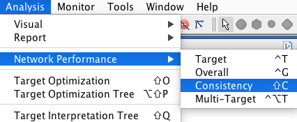
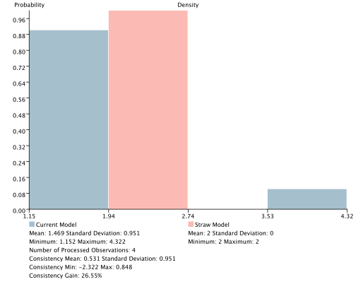
This feature compares two density graphs, with the x-axis representing the log-likelihood of the n-dimensional evidence sets stored in the dataset(s) associated with the current network:
- the blue bars correspond to the reference model,
- the red bars correspond to the straw model.
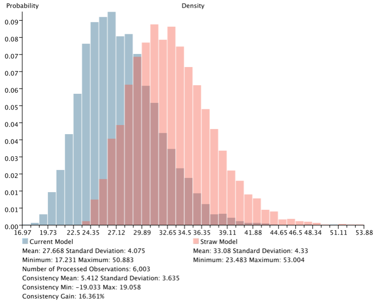
If the reference model is a good representation of the joint probability distribution sampled by the evidence contained in the associated dataset, the blue bars should be to the left and clearly separated from the red bars. Bars further to the left on the x-axis indicate lower log-likelihood values, which imply higher joint probabilities.
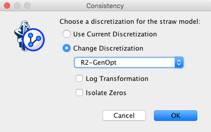
As before, the straw model is the fully unconnected network. However, if the network contains discretized variables, we have a choice regarding the discretization. We can either keep the same discretization for both networks, or choose an alternative discretization algorithm for the straw model, with the requested number of bins being the same as the number of bins in the reference model.
Beyond the graphical comparison, the following Consistency Gain can be used to quantify the discrepancy between the reference model () and the straw model ():
for the evidence , and
for the entire data set, where is the number of rows.
Example
Again, we use the simple reference structure with 2 boolean nodes, and .
Strong Dependency
Here, the associated dataset contains the 4 different weighted pieces of evidence that can be generated from the joint probability distribution represented by the reference model.

| Evidence | Joint Probability - Reference | Joint Probability - Straw | Log-Likelihood - Reference | Log-Likelihood - Straw |
|---|---|---|---|---|
| E1 | 0.45 | 0.25 | 1.152 | 2 |
| E2 | 0.05 | 0.25 | 4.322 | 2 |
| E3 | 0.05 | 0.25 | 4.322 | 2 |
| E4 | 0.45 | 0.25 | 1.152 | 2 |
| Consistency Mean | 0.531 |
Weak Dependency
Here, the associated dataset contains the 4 different weighted pieces of evidence that can be generated from the joint probability distribution represented by the reference model.

| Evidence | Joint Probability - Reference | Joint Probability - Straw | Log-Likelihood - Reference | Log-Likelihood - Straw |
|---|---|---|---|---|
| E1 | 0.275 | 0.25 | 1.862 | 2 |
| E2 | 0.225 | 0.25 | 2.152 | 2 |
| E3 | 0.225 | 0.25 | 2.152 | 2 |
| E4 | 0.275 | 0.25 | 1.862 | 2 |
| Consistency Mean | 0.007 |

New: Relationship Analysis Report
As shown above, the Consistency Mean offers a good way to express the strength of the dependencies represented by the reference model. However, this metric can only be computed if data is available to sample the joint probability distribution.
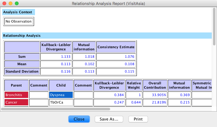
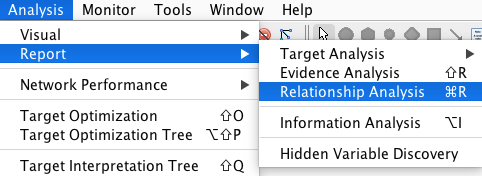
If no data is associated with the model, the Consistency Mean can be efficiently approximated by computing the average of the sum of all Arc Forces (Kullback-Leibler Divergence) and the Mutual Information between all pairs of nodes that are connected by an arc. This Consistency Estimate is available in the first part of the Relationship Analysis Report:
