
Numerical Evidence
Context
Instead of a specific probability distribution, an observation or scenario may exist in the form of a single numerical value, which means that we need to set Numerical Evidence. For instance, a stock market analyst may wish to examine how other stocks performed given a hypothetical period of time during which the average of the daily returns of JNJ was −1%. Naturally, this requires that we set evidence on JNJ that has an expected (mean) value of −0.01 (=−1%). However, this task is not as straightforward as it may sound; the question will become apparent as we go through the steps to set this evidence.
Usage
Select the Monitor of node , then select Node Contextual Menu > Enter Numerical Evidence. Next, we type “−0.01” into the dialog box for Target Mean/Value.
Observation Type
Additionally, as was the case with Probabilistic Evidence, we have to choose the type of validation, but we now have three options under Observation Type:
No Fixing, the same as the green button, i.e., validation with static likelihood.Fix Mean, where the likelihood is dynamically computed to maintain the mean value, although the probability distribution can change as a result of setting additional evidence. In an evidence scenario file, a fixed mean is stored with the notationm{...}.Fix Probabilities, i.e., validation with dynamic likelihood. In an evidence scenario file, fixed probabilities are stored with the notationp{...}.
Fixing the mean or probabilities is only valid for exact inference; with approximate inference there is no convergence algorithm.
Distribution Estimation Methods
Apart from setting the validation method, we also need to choose the Distribution Estimation Method, as we need to come up with a distribution that produces the desired mean value. There are a great number of distributions that could potentially produce a mean value of −0.01; to make a prudent choice, we first need to understand what the evidence represents. Only then can we choose from the three available algorithms for generating the Target Distribution:
Special Cases of Numerical Evidence
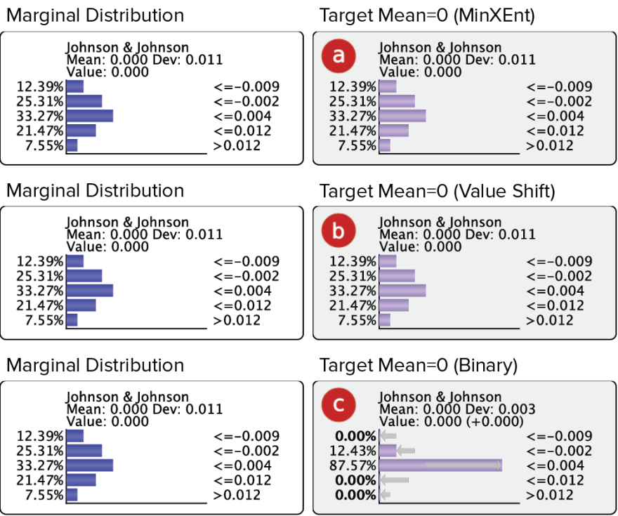
If the Numerical Evidence is equal to the current expected value, using MinXEnt (a) or Value Shift (b) will not change the distribution. Using the Binary algorithm (c), however, will return a different distribution (except in the context of a binary node).
Example: Conflicting Evidence
In the examples shown so far, setting evidence typically reduced uncertainty with regard to the node of interest. However, this is not always the case: occasionally, separate pieces of evidence can conflict with each other. We illustrate this by setting Numerical Evidence (using MinXEnt) on JNJ and KMB, starting from the marginal distribution.

After setting Numerical Evidence (using MinXEnt) with a Target Mean/Value of +1.5% on JNJ, the posterior probabilities indicate that the PG distribution is more positive than before, and the uncertainty regarding PG is lower. In the KMB Monitor, the gray arrows and ”(+0.004)” indicate that this first evidence increases the expectation that KMB will also increase in value.

If we then observe that KMB decreased by 1.5% (again using MinXEnt), this goes against our expectations.

The result is a more uniform probability distribution for PG, rather than a narrower one, increasing our uncertainty about PG compared to the marginal distribution. Even though it appears we have “lost” information, we may have a knowledge gain after all: the increased uncertainty can be interpreted as a higher expectation of volatility.