Parameter Estimation

Now we can see the real benefit of bringing all variables as nodes into BayesiaLab. To calculate Mutual Information, all the terms of the equation $I(X,Y)=H(X)-H(X \mid Y)$ can be easily computed with BayesiaLab once we have a fully specified network.

We start with a pair of nodes, namely $\mathit{Neighborhood}$ and $\mathit{SalePrice}$. As opposed to $\mathit{LotArea}$, which is a discretized Continuous variable, $\mathit{Neighborhood}$ is categorical, and, as such, it has been automatically treated as Discrete in BayesiaLab. This is the reason the node corresponding to $\mathit{Neighborhood}$ has a solid border. We now add an arc between these two nodes to explicitly represent the dependency between them:

Click to Zoom

×

The yellow warning triangle reminds us that the Conditional Probability Table (CPT) of $\mathit{SalePrice}$ given $\mathit{Neighborhood}$ has not been defined yet. In Chapter 4, we defined the CPT based on existing knowledge. On the other hand, as we have an associated database, BayesiaLab can use it to estimate the CPT by using Maximum Likelihood, i.e., BayesiaLab “counts” the (co-)occurrences of the states of the variables in our data. The table below shows the first 10 records of the variables $\mathit{SalePrice}$ and $\mathit{Neighborhood}$ from the Ames dataset.

Counting all records, we obtain the marginal count of each state of $\mathit{Neighborhood}$.

Given that our Bayesian network structure says that $\mathit{Neighborhood}$ is the parent node of $\mathit{SalePrice}$, we now count the states of $\mathit{SalePrice}$ conditional on $\mathit{Neighborhood}$. This is simply a cross-tabulation.

Once we translate these counts into probabilities (by normalizing by the total number of occurrences for each row in the table), this table becomes a CPT. Together, the network structure (qualitative) and the CPTs (quantitative) comprise the Bayesian network.

In practice, however, we do not need to bother with these individual steps. Rather, BayesiaLab can automatically learn all marginal and conditional probabilities from the associated database. We select Menu > Learning > Parameter Estimation to perform this task.

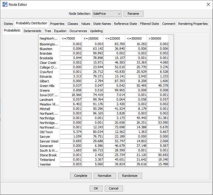
Upon completing the Parameter Estimation, the warning triangle has disappeared, and we can verify the results by double-clicking $\mathit{SalePrice}$ to open the Node Editor. Under the tab Probability Distribution > Probabilistic we can see the probabilities of the states of $\mathit{SalePrice}$ given $\mathit{Neighborhood}$. The CPT presented in the Node Editor is indeed identical to the table shown above.

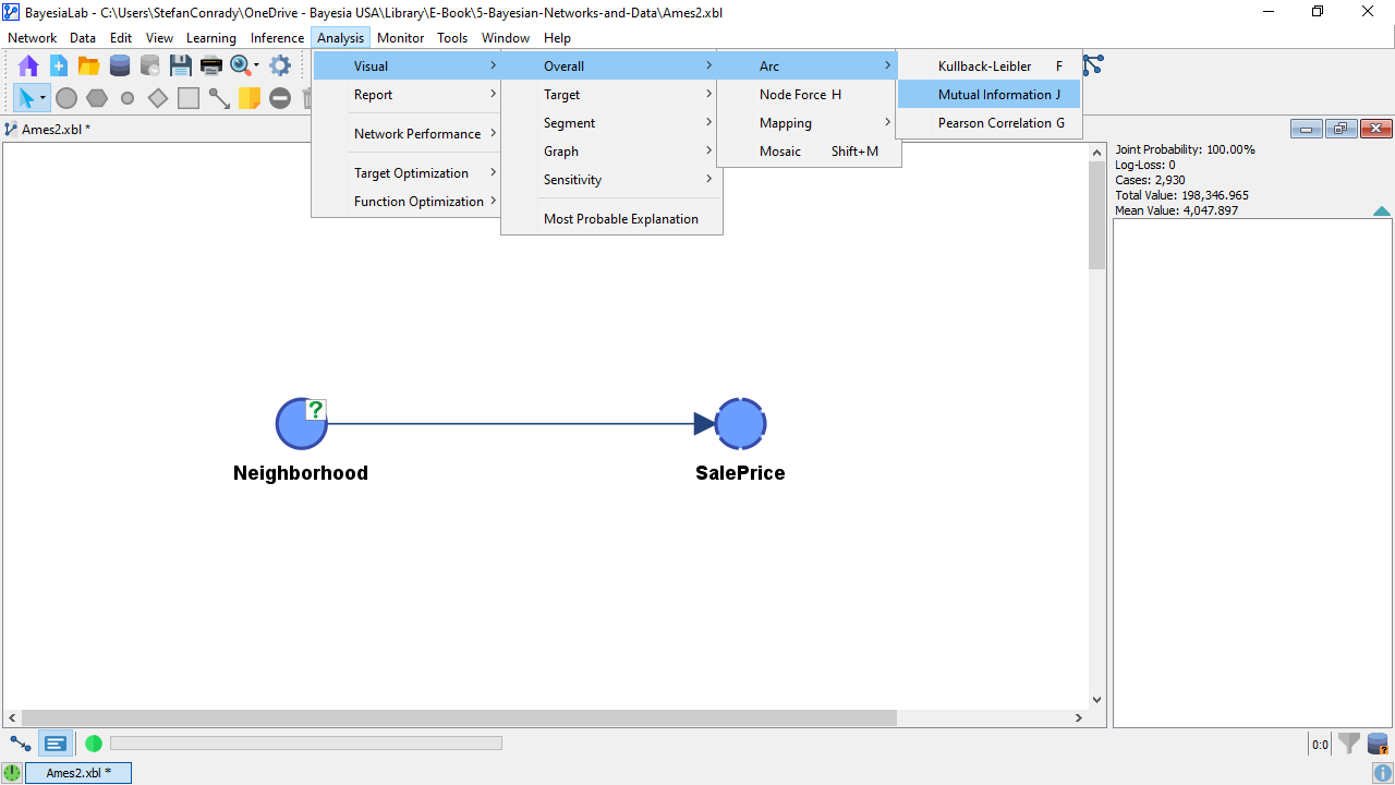
This model now provides the basis for computing the Mutual Information between $\mathit{Neighborhood}$ and $\mathit{SalePrice}$. BayesiaLab computes Mutual Information on demand and can display its value in numerous ways. For instance, in Validation Mode F5, we can select Menu > Analysis > Visual > Arc > Overall > Mutual Information.

Click to Zoom

×

The value of Mutual Information is now represented graphically in the thickness of the arc. This does not give us much insight because we only have a single arc in this network. So, we click the Show Arc Comments icon in the Toolbar to show the numerical values.

Click to Zoom

×

The top number in the Arc Comment box shows the actual Mutual Information value, i.e., 0.6462 bits. We should also point out that Mutual Information is a symmetric measure. As such, the amount of Mutual Information that $\mathit{Neighborhood}$ provides on $\mathit{SalePrice}$ is the same as the amount of MI that $\mathit{SalePrice}$ provides with regard to $\mathit{Neighborhood}$. This means that knowing the $\mathit{SalePrice}$ reduces the uncertainty with regard to $\mathit{Neighborhood}$, even though that may not be of interest.

Without context, however, the value of Mutual Information is not meaningful. Hence, BayesiaLab provides an additional measure, i.e., the Symmetric Normalized Mutual Information, which gives us a sense of how much the entropy of $\mathit{SalePrice}$ was reduced. Previously, we computed the marginal entropy of $\mathit{SalePrice}$ to be 1.85. Dividing the Mutual Information by the Marginal Entropy of $\mathit{SalePrice}$ gives us a sense of how much our uncertainty is reduced:

$\displaystyle \frac{0.5999}{1.85} = 0.3243 = 32.43\%$

Conversely, the red number shows the Relative Mutual Information with regard to the parent node, $\mathit{Neighborhood}$. Here, we divide the Mutual Information, which is the same in both directions, by the Marginal Entropy of $\mathit{Neighborhood}$:

$\displaystyle \frac{0.5999}{4.1839} = 0.1434 = 14.34\%$

This means that by knowing $\mathit{Neighborhood}$, we reduce our uncertainty regarding $\mathit{SalePrice}$ by 32% on average. By knowing $\mathit{SalePrice}$, we reduce our uncertainty regarding $\mathit{Neighborhood}$ by 14% on average. These values are readily interpretable. However, we need to know this for all nodes to determine which node is most important.