Most Relevant Explanations (9.0)

Context

This feature uses a genetic algorithm for searching partial instantiations of sets of variables that maximize the Generalized Bayes Factor (GBF) as the best explanations for a given set of evidence.

It is mainly based on the article written by Yuan, C. et al. (2011), “Most Relevant Explanations in Bayesian Networks ”, Journal of Artificial Intelligence Research, pp. 309-352.

The Weight of Evidence (WoE), the logarithm of the GBF, dates back to work by Alan Turing in World War II (see Good, I. J. (1985), “Weight of Evidence: A Brief Survey ”, Bayesian Statistics 2, pp. 249-270, for more general discussion of history and concepts):

$\displaystyle WoE(E, H) = \log_2 \left( GBF(E, H) \right)$

where

• $E$ represents the current set of evidence (any type of evidence on any number of variables) for which we are seeking concise and precise explanations, and
• $H$ is the hypothesis described with hard evidence on a subset of variables

$\displaystyle GBF(E, H) = \frac{P(E \mid H)}{P(E \mid \overline{H})} = \frac{O(H \mid E)}{O(H)}$

where $\overline{H}$ is the negation of $H$, and $O(\cdot)$ denotes the odds:

$\displaystyle O(H) = \frac{P(H)}{P(\overline{H})}$

$\displaystyle O(H \mid E) = \frac{P(H \mid E)}{P(\overline{H} \mid E)}$

As we can see, the GBF is expressed with two equivalent terms:

$\displaystyle \frac{P(E \mid H)}{P(E \mid \overline{H})}$, a likelihood ratio,

$\displaystyle \frac{O(H \mid E)}{O(H)}$, an odds ratio.

Even though they are strictly equivalent, the likelihood ratio is a natural interpretation of the GBF when the explanation $H$ you are looking for belongs to the Ancestors of $E$ in your Causal Bayesian Network (i.e. you assume that all arcs are in the causal direction and do not represent mere associations).

On the other hand, you can interpret the GBF as an odds ratio either when your network is not causal, or when the explanation $H$ you are looking for does not belong exclusively to the Ancestors of $E$.

Usage

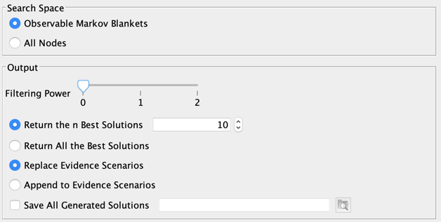
Select Menu > Analysis > Report > Evidence > Most Relevant Explanations

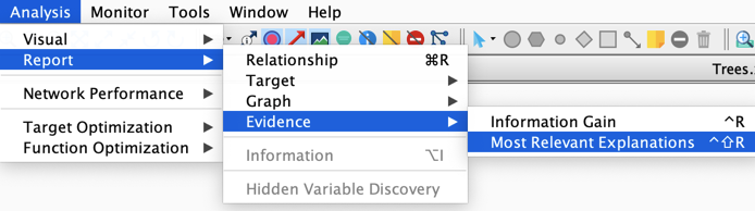
The following wizard will help you set the options you want to use for searching the most relevant explanations of your current set of evidence $E$.

It consists of four main sections.

1. Search Space

This defines which nodes will be included in the search. The nodes that belong to $E$ and those that are Not Observable are excluded from the search. There are 4 options:

• The Selected Nodes,
• The nodes that belong to the Observable Markov Blanket(s) of the $E$,
• The Ancestors of $E$,
• All Nodes.

The choice of the Ancestors option only makes sense when your network is causal.

2. Output

There are different available options for setting the output (Report and Evidence Scenario File):

• Filtering Power:
  • 0: All solutions are reported,
  • 1: The Strongly Dominated solutions are excluded from the report. $H_s$ is strongly dominated by $H_d$, a dominant explanation when $H_s \supset H_d$ and $GBF(H_d) \ge GBF(H_s)$,
  • 2: The Strongly and Weakly Dominated solutions are excluded from the report. $H_w$ is weakly dominated by $H_d$, when $H_w \subset H_d$ and $GBF(H_d) \gt GBF(H_w)$,
• Return the n Best Solutions: returns only a subset of (filtered) solutions,
• Return All the Best Solutions: returns all (filtered) solutions,
• Replace Evidence Scenarios: replaces your current scenarios with the returned explanations,
• Append to Evidence Scenarios: adds the return explanations to your current evidence scenarios,
• Save All Generated Solutions: saves all (unfiltered) explanations in a file.

3. Genetic Settings

The BayesiaLab’s MRE feature is using our genetic algorithm for searching the best explanations. This genetic algorithm can be customized:

• Number of Kingdoms: number of populations that evolve independently,
• Population Size: number of individuals/solutions per population,
• Crossover Rate: the probability for the individuals of the worst kingdom to be generated by crossing the genes of the best individuals of two randomly selected kingdoms,
• Gene Mutation Rate: the probability to mute a gene of an individual,
• Selection Rate: the probability for an individual to be selected to breed the new generation,
• Fixed Seed: this algorithm being stochastic, using a fixed seed allows you to reproduce your results.

Clicking allows you to go back to the default settings.

The iconsin the upper right corner allows you to show and hide these options respectively.

4. Genetic Stop Criterion

The genetic algorithm is an anytime algorithm that can run forever. If you do not want to stop it manually by clicking in the lower-left corner of the graph window, you can define a stop criterion based on the consecutive number of generations without any improvement. The number of generations without improvement can be calculated at the kingdom level or across all kingdoms.

Clicking allows you to go back to the default settings.

The icons in the upper right corner allow you to show and hide these options respectively.

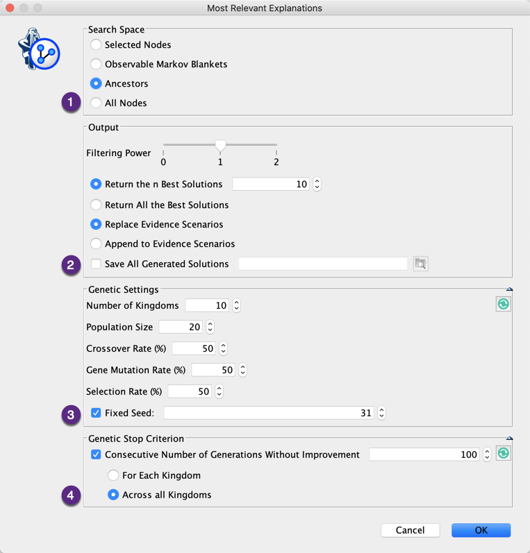
Example 1: Fault Diagnosis

For illustration, we use Causal Bayesian Network corresponding to an electrical circuit. $A$, $B$, $C$, and $D$ are switches. In working order, all switches are open. As a result, there is no current flowing through the $Output$, i.e., $\mathit{Output} = \mathit{No\ Current}$.

Click to Zoom

×

This example is described in Yuan et al. (2011) and was originally suggested by Poole and Provan (1991). Poole and Provan’s work appears in What Is the Most Likely Diagnosis?, in Bonissone, P., Henrion, M., Kanal, L., and Lemmer, J. (eds.), Uncertainty in Artificial Intelligence 6, pp. 89–105. Elsevier Science Publishing Company, New York, NY.

The default, non-defective condition of this network is shown below.

Click to Zoom

×

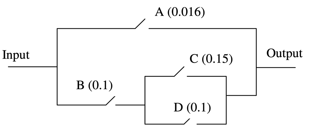
Now we observe a failure mode, which means that there is a current going through the $Output$, i.e., $\mathit{Output} = \mathit{Current}$.

Our task is to find the “most relevant explanations” for the failure of this system. More specifically, we want to find the defective switch or switches, which cause the overall failure.

We first set the nodes that represent the local outputs to Not Observable, and furthermore set $\mathit{Output} = \mathit{Current}$.

Click to Zoom

×

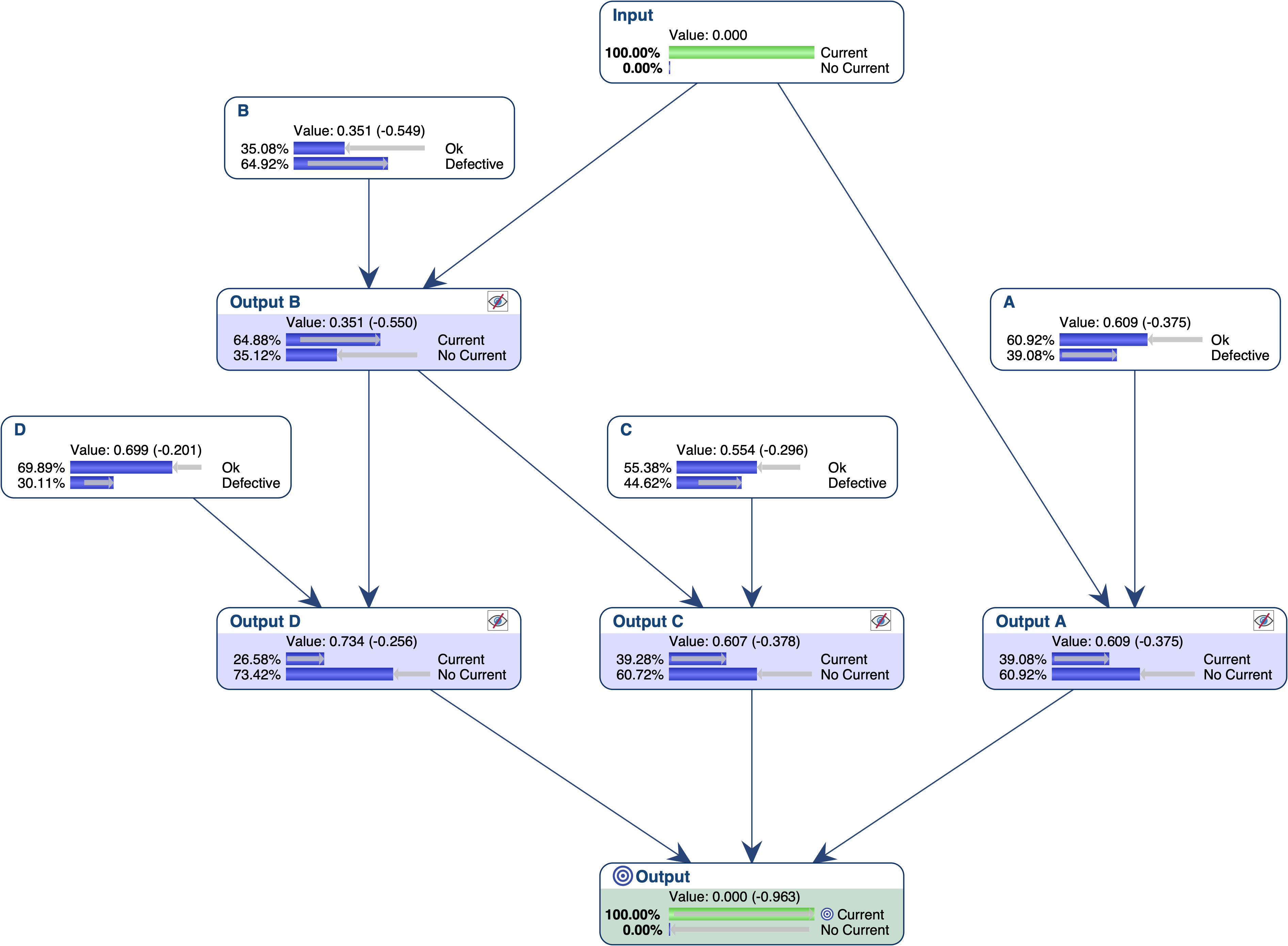
The most relevant explanation $H$ for observing evidence $E$, which is $\mathit{Output} = \mathit{Current}; \mathit{Input} = \mathit{Current}$, is that switches $B$ and $C$ are defective.

Click to Zoom

×

In addition to reporting the Most Relevant Explanation, the table contains six measures:

• MRE Size: the number of observations in $H^{*}$. $H^{*}$ consists of two pieces of evidence, $B$ and $C$.
• Weight of Evidence: the binary logarithm of the Generalized Bayes Factor
• Generalized Bayes Factor
• Likelihood $P(E \mid H)$
• Posterior Odds $O(H \mid E)$
• Posterior Probability $P(H \mid E)$

Since our model is causal, we can use the likelihood ratio for interpreting the GBF. The likelihood that $B$ and $C$ are defective is the cause of $E$ is 42 times greater than the likelihood that ”$B$ or $C$ are okay” is the cause of $E$ (48.4% versus 1.1%).

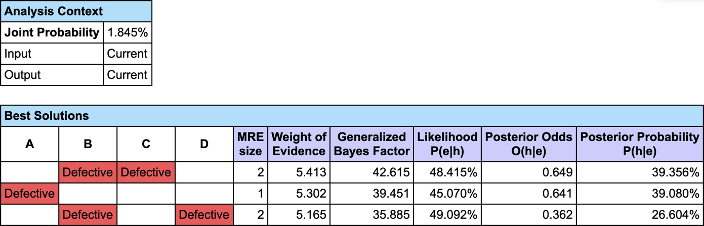
Filter 0

Click to Zoom

×

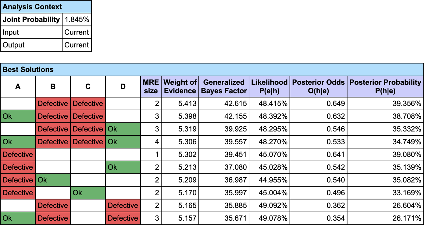
Filter 1: Strongly Dominated

Click to Zoom

×

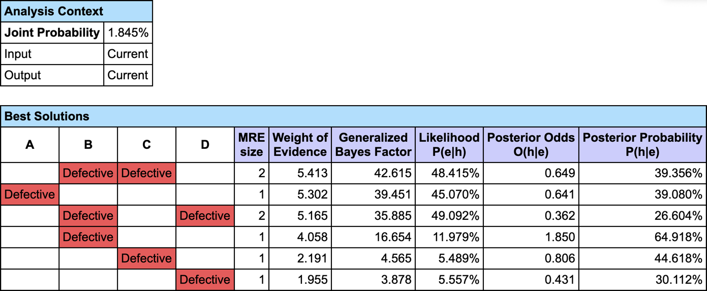
Filter 2: Strongly and Weakly Dominated

Click to Zoom

×

Example 2: MRE for Cluster Interpretation

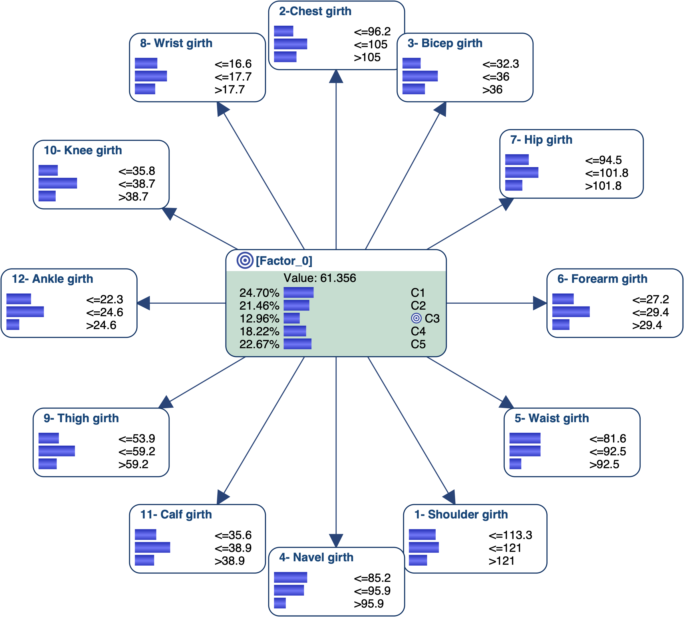
Let’s suppose we have a data set that describes physically active men (several hours of exercise a week) with body girth measurements and skeletal diameter measurements. We used Data Clustering in order to automatically create a latent variable that represents a typology of these men and found 5 clusters.

We know need to interact with the Bayesian network to try to associate an image/name with each state of the latent variable. We can obviously use the monitors and manually set evidence on each state of [Factor_0] to analyze the posterior probability distributions of all measurements. We can also use some tools that will automatically set evidence on the target node [Factor_0] or on the measurements.

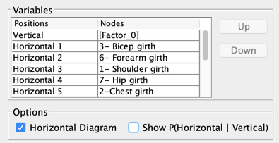
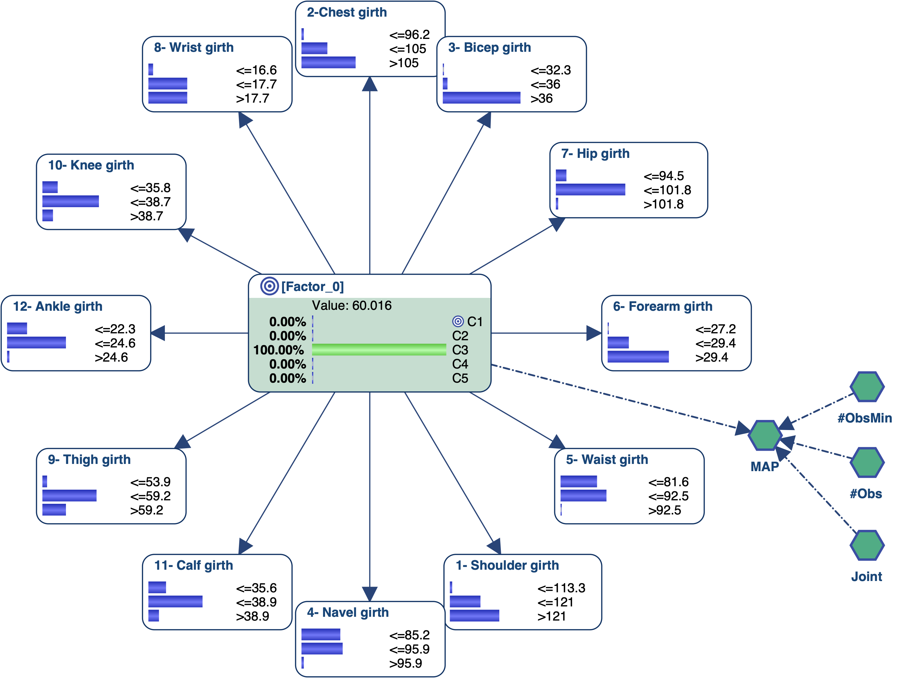
Let’s try to get the profile of the men that are associated with C3 and represent 13% of the overall population. We set C3 as the Target State.

Click to Zoom

×

Measurements’ Posterior

We can sort the monitors with respect to their correlation with C3 (Monitor | Sort | Target State Correlation, or via the Monitor Pane Contextual menu)

and then set a Hard Evidence on C3

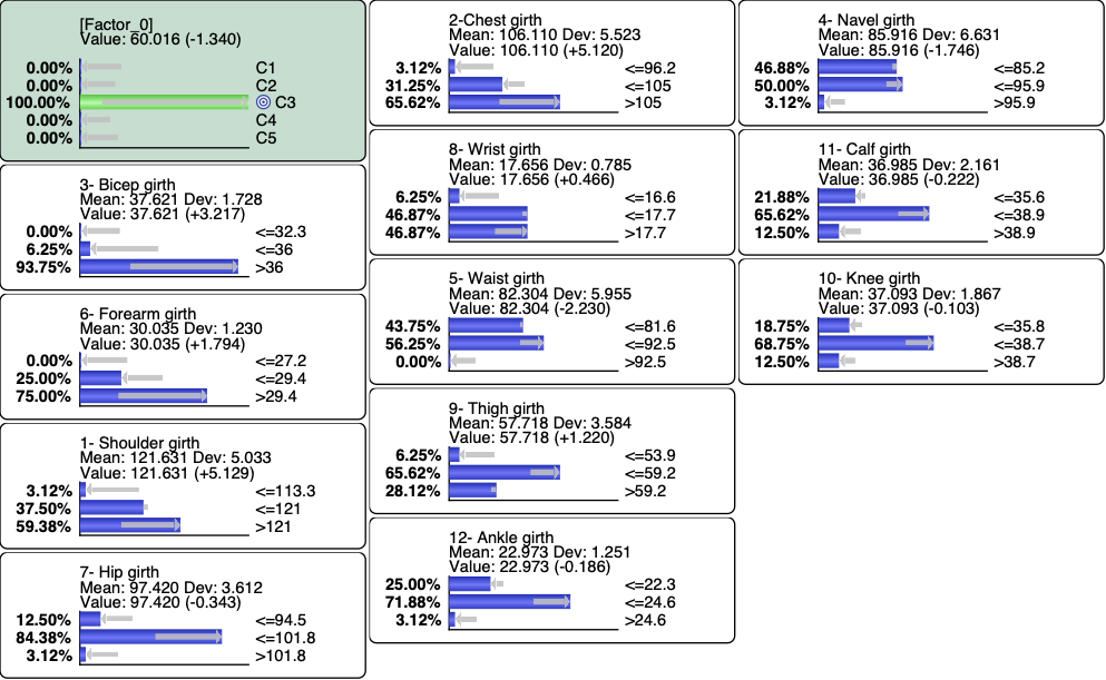
We can also use the Monitor Contextual menu to highlight the variations.

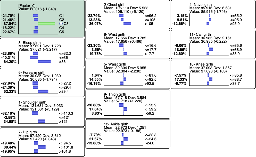
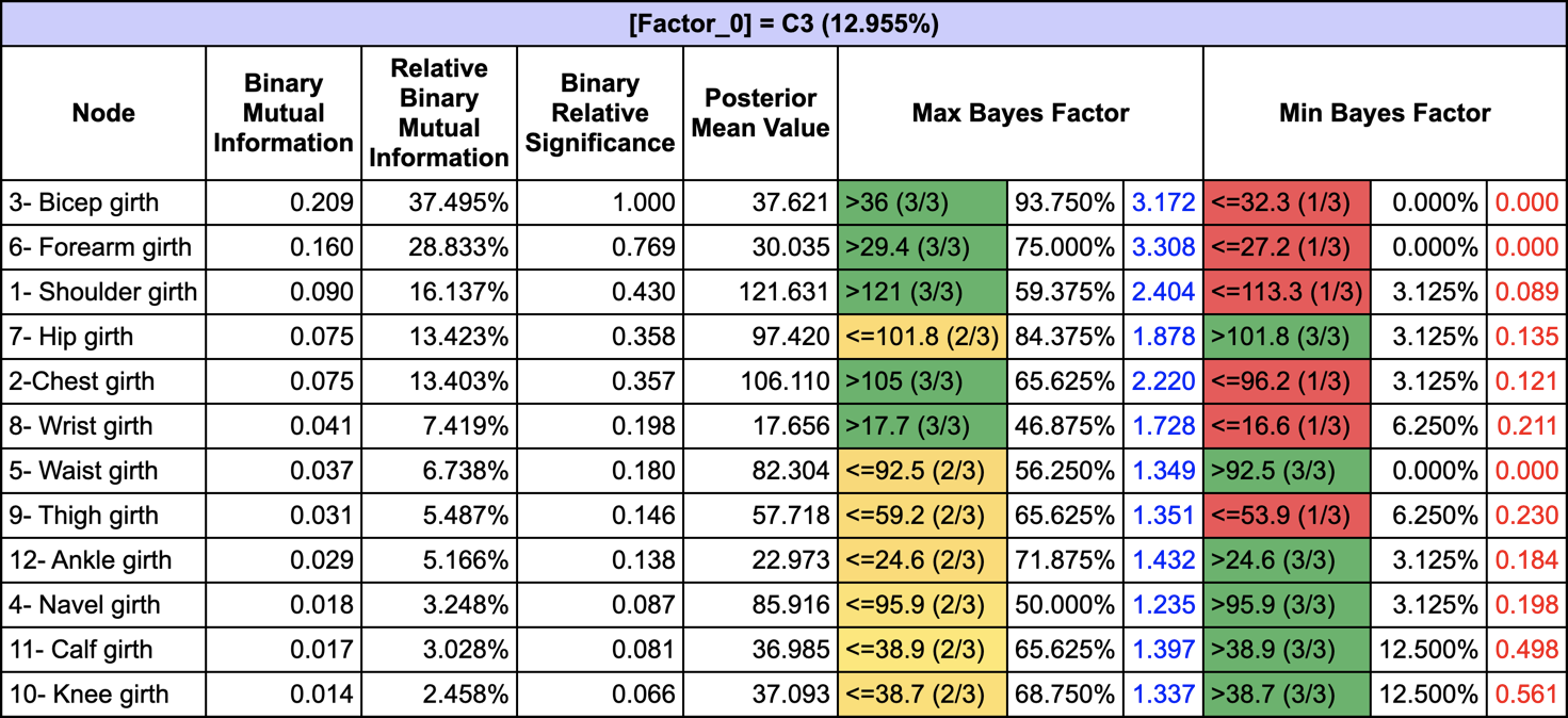
Relationship with Target

The Relationship with Target Node (Analysis > Report > Target > Relationship with Target Node) allows us to get all the posterior probabilities given C3 along with the Maximum and Minimum Bayes Factors:

Click to Zoom

×

Mosaic

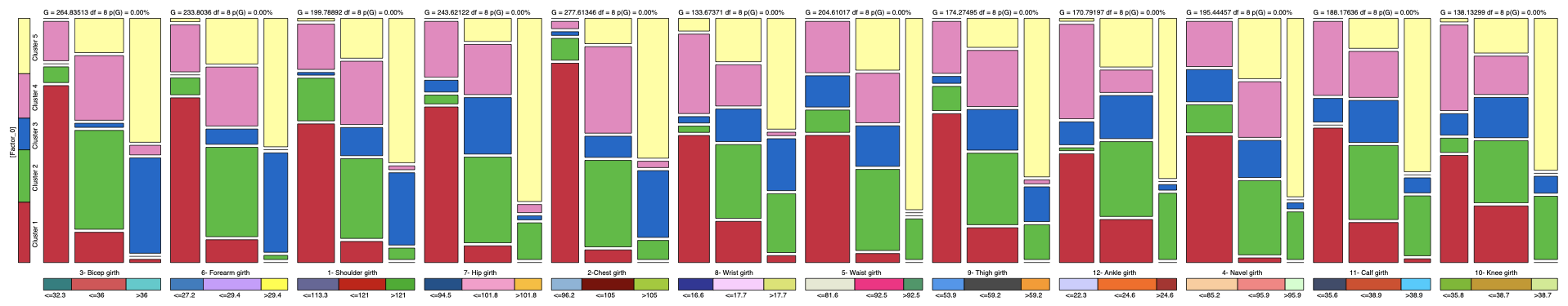
The Mosaic Analysis (Analysis | Visual | Overall | Mosaic) returns a graph with the posterior probability distributions of all measurements given each cluster:

Click to Zoom

×

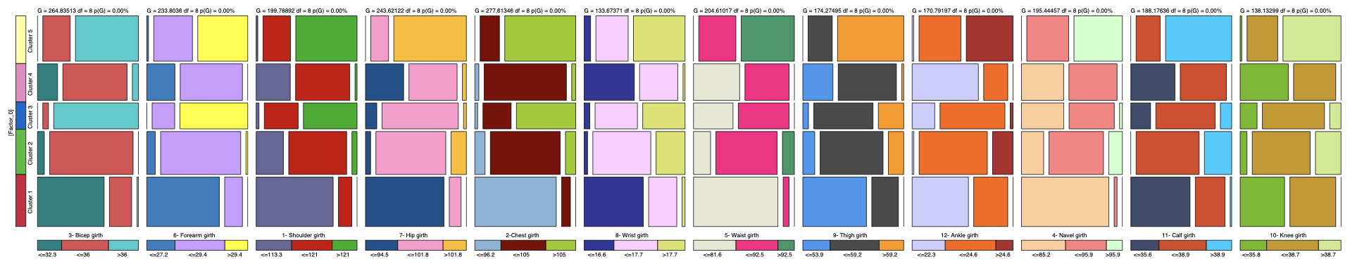
The posterior distributions that correspond to C3 are represented in the third row of each block.

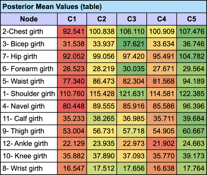
Posterior Mean Values

Since the measurements are numerical, we can analyze their Posterior Mean Values given each cluster (Report | Target | Posterior Mean Analysis):

and generate the corresponding Radar Chart to visually compare the mean values given C3 with the prior values (i.e. on the entire population).

Click to Zoom

×

Note that we can get a similar Radar by using the Segment Profile Analysis that we introduced in version 8.0 (Analysis | Visual | Segment | Profile):

Click to Zoom

×

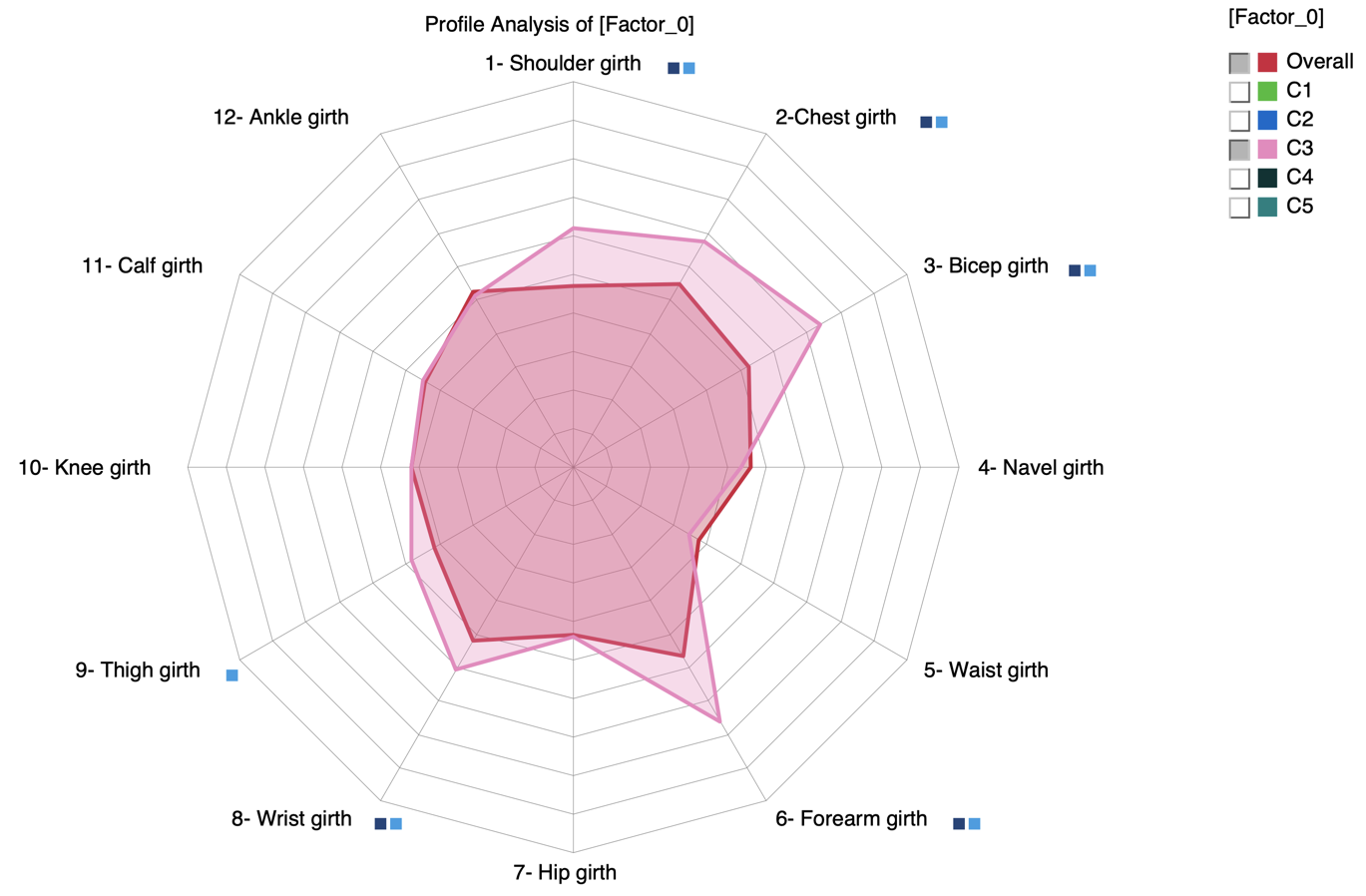
A square is added next to the label when the mean values of the Overall population and C3 are estimated as significantly different

• for t-test (Frequentist)
• for BEST (Bayesian)

Clusters’ Posterior

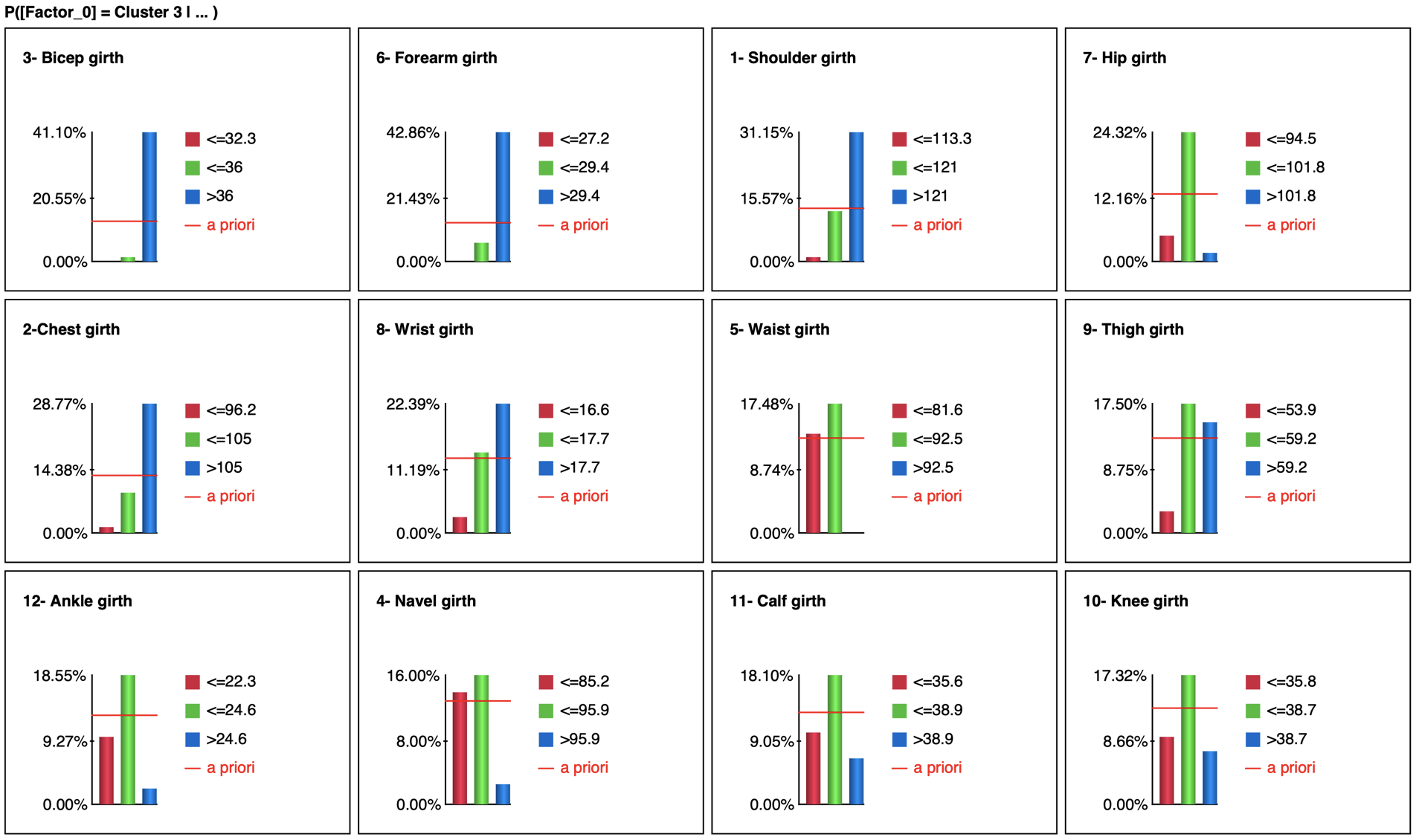
We can also analyze C3 by setting evidence on the measurements. This can be done efficiently by using Histograms (Analysis | Visual | Target | Target’s Posterior | Histograms):

Click to Zoom

×

Tornado

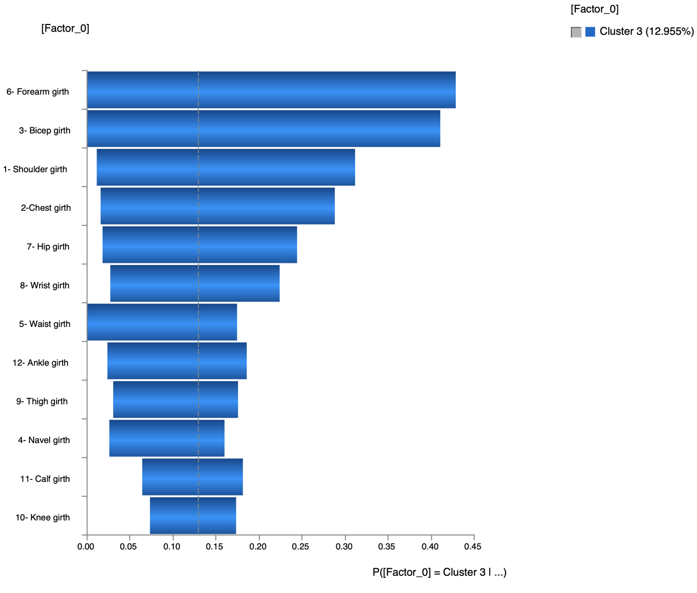
The Tornado (Analysis | Visual | Target | Target’s Posterior | Tornado Diagrams | Total Effects) shows the impact on the probability of C3 when setting evidence on each measurement

Click to Zoom

×

We can also use the Mosaic Analysis (Analysis > Visual > Overall > Mosaic) to get posterior probability distributions of the Target node given each state of the measurements:

Click to Zoom

×

where the posterior probability of C3 is represented in blue.

Optimization

All the previous methods to analyze C3 are based on 1-piece of evidence (either set on the cluster or on the measurements). We can use the BayesiaLab’s optimization tools to work with more complex evidence.

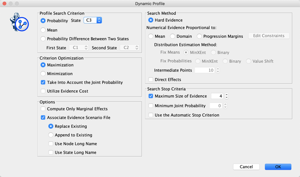
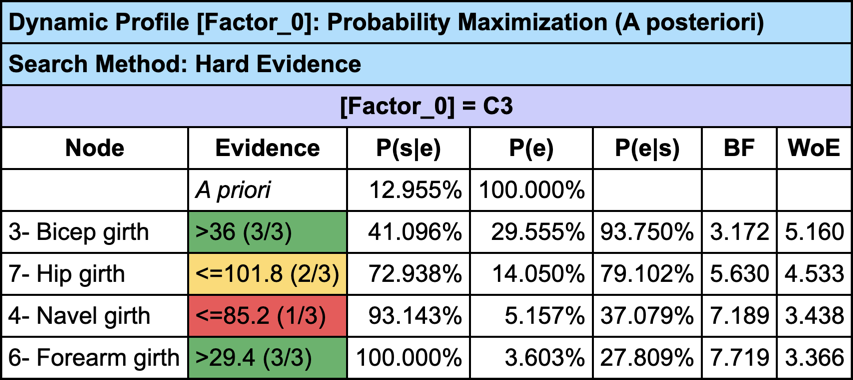
Dynamic Profile

The Dynamic Profile is a greedy search algorithm that we can use here to create a profile that describes the men associated with C3:

Tree

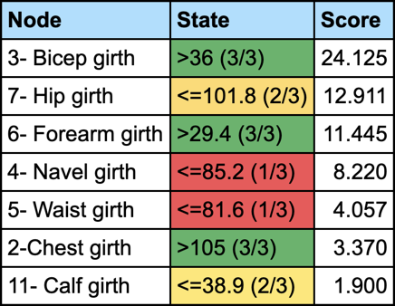
Instead of just using a greedy search for creating the profile of C3, we can use the Target Optimization Tree to create a set of “sketches”:

Click to Zoom

×

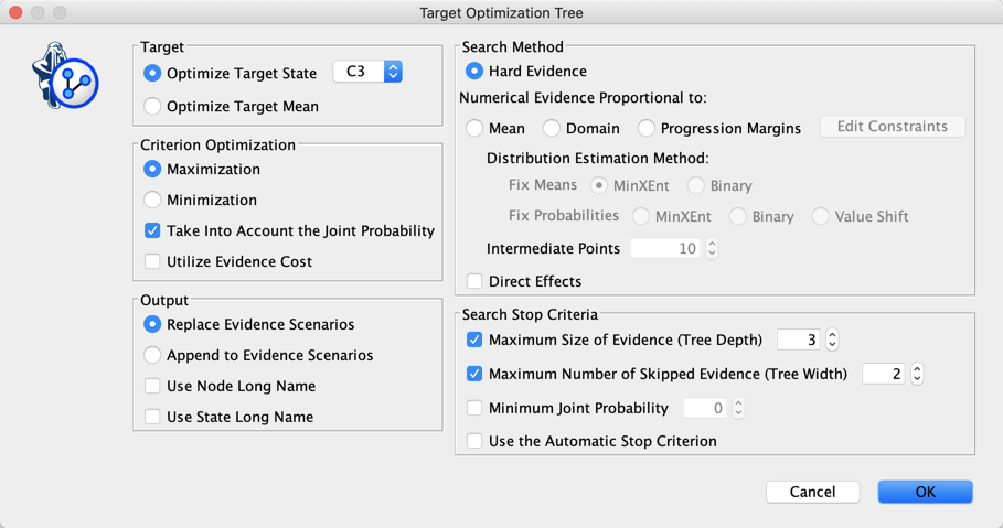
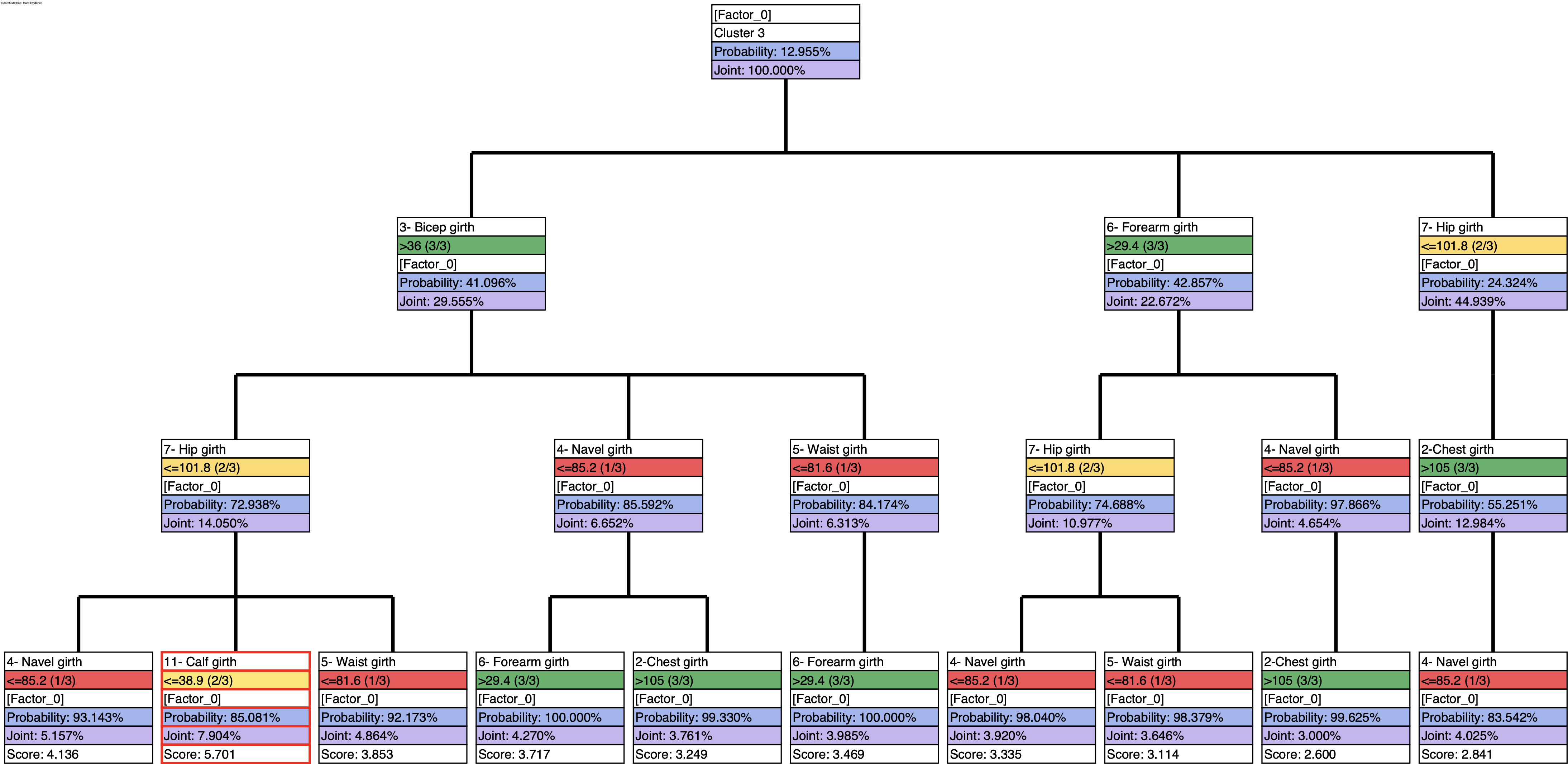
and then generate the report that summarizes the weight of each trait in these sketches:

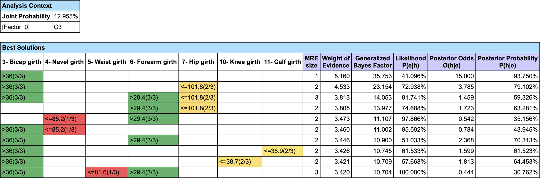
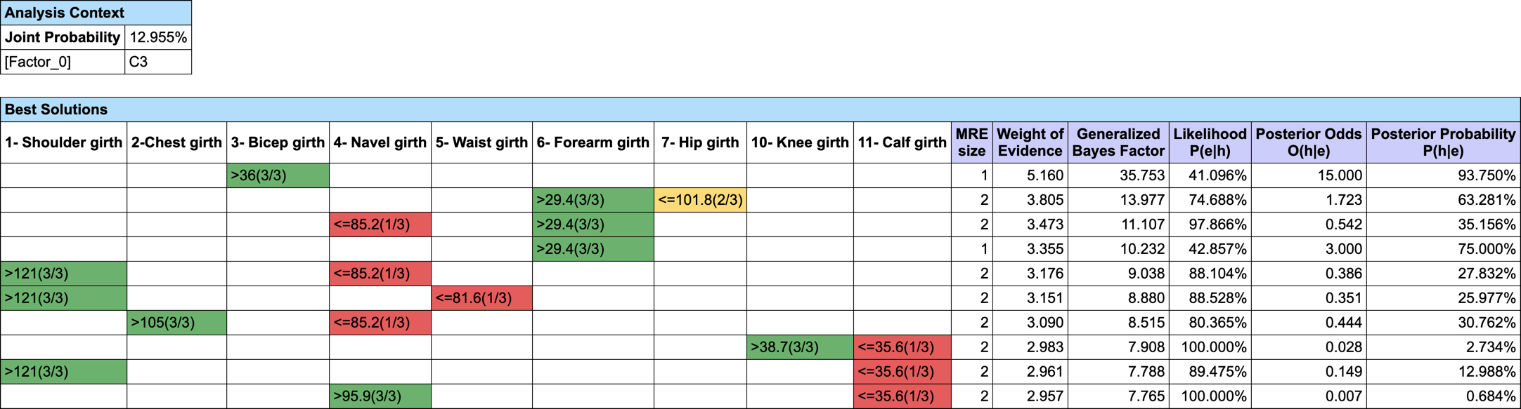
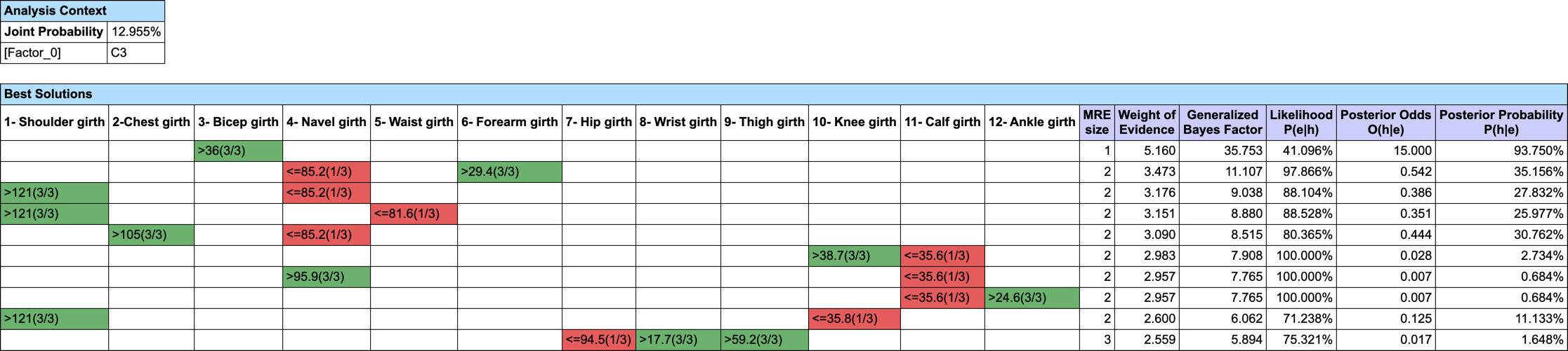
MRE

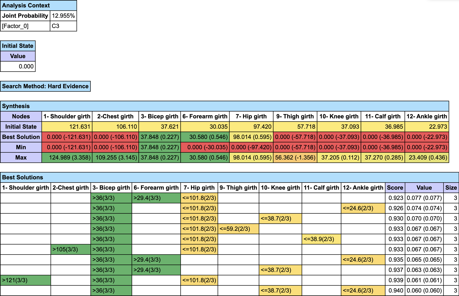
We first set the evidence on C3 and then run Most Relevant Explanations.

The most relevant explanation H* for the evidence $E={[Factor_0]}$ is 3- Bicep girth > 36cm (the 3rd and last state)

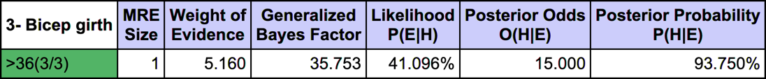
Since the context of profiling a latent variable is not causal, we interpret the Generalized Bayes Factor with the Odds ratio: the conditional odds of 3- Bicep girth > 36cm given C3 are almost 36 times greater than the marginal odds (15 versus 0.42).

Filter 0

Click to Zoom

×

Filter 1: Strongly Dominated

Click to Zoom

×

Filter 2: Strongly and Weakly Dominated

Click to Zoom

×

MAP

Let’s suppose we want to find out what are the triplets of traits that Maximize the A Posteriori given C3. We do not have (yet) a MAP function implemented in BayesiaLab, but we can easily augment our Bayesian network with Function Nodes and use our Genetic Function Optimization tool to find our triplets (Analysis | Function Optimization | Genetic).

Click to Zoom

×

• #Obs: the number of Hard Evidence set in the network. We can get this number with the Inference Function ObsCount(True, false, false, false),
• #ObsMin: the minimum number of Hard Evidence that we set to 4 to search for triplets (i.e. C3 plus the triplets),
• Joint: the joint probability of the current set of evidence. It is returned by the Inference Function JointProb(),
• MAP: the score we want to maximize, defined with the equation if $(?\#\text{Obs}?<?\#\text{ObsMin}?, 0, ?\text{Joint}?)$.

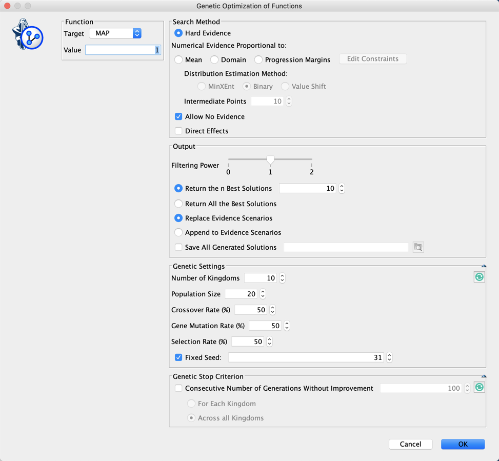
We did not set here any Stop Criterion. This means that we will need to stop the genetic algorithm by clicking in the lower-left corner of the graph window.

The current Best Score is shown at the end of the Progress Bar. You can also see which Generation found this score.

You can also see at the lower right corner of the Graph Panel the icon blinking. This indicates that there are some outputs in the Console. Clicking on this icon will open the Console:

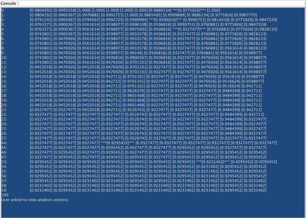
While the first column indicates the Generation, the following columns return the score of the current best individual in each Kingdom. When a score is framed with ”***”, it indicates that there has been an improvement in this Generation

Click to Zoom

×

If you want to find out the MAP on a specific subset of nodes, you just have to set #ObsMin to 0, and either select the nodes before running the optimization with “Restrict Search to the Selected Nodes”, or set all other nodes as Not Observable.

Here is an image that represents the profile of the men who belong to C3 on the basis of all these analyses: