Causal Effect Estimation in BayesiaLab with Graph Surgery
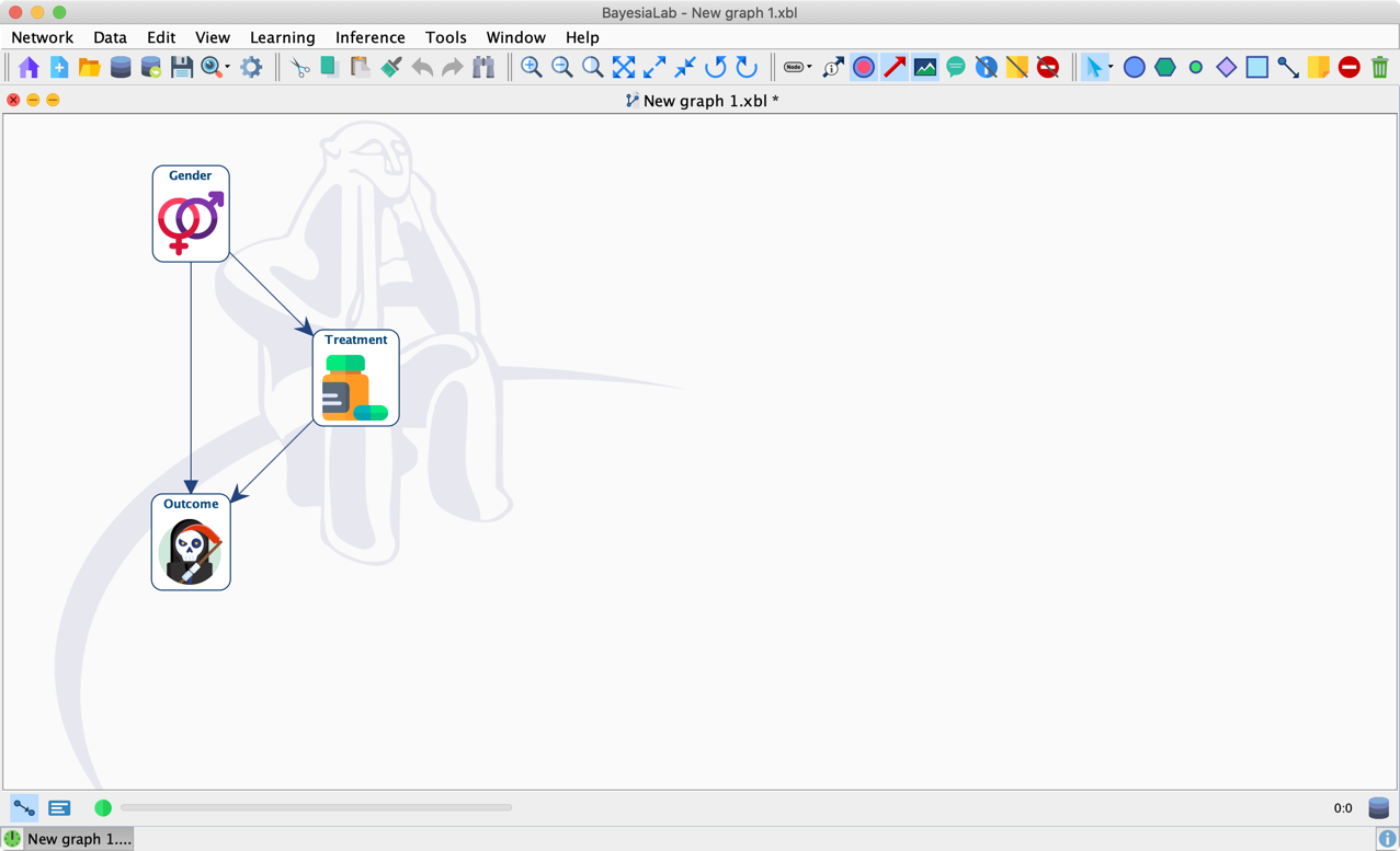
We now understand that Graph Surgery and Adjustment are equivalent. However, with Bayesian networks, we can go beyond the metaphor and—quite literally—perform graph surgery. In this section, we create a Bayesian network to represent Simpson’s Paradox example and then perform graph surgery to estimate the causal effect.
We have already defined a causal graph earlier when we encoded our causal assumptions regarding this domain. We can reuse this causal understanding for building a causal Bayesian network in BayesiaLab.
As we illustrated in the context of the knowledge modeling exercise in Chapter 4, we manually create the nodes and draw the arcs on BayesiaLab’s Graph Panel. We choose to use long names for the nodes instead of X, Y, and Z. Letters were very convenient for formulas, but long names increase the readability of Bayesian networks. To further help with interpretation, we also associate images with each node and display them as Badges. Then, we select Menu > View > Layout > Genetic Grid Layout > Top-Down Repartition to obtain a layout that takes into account the direction of the arcs and define layers accordingly.
The Genetic Grid Layout algorithms are particularly useful for causal networks. We can, therefore, define one of these two algorithms as the one associated with the shortcut P via Menu > Preferences > Window > Preferences > Automatic Layout > Layout Algorithm Associated with Shortcut.

The yellow warning symbols remind us that the probability tables associated with the nodes have yet to be defined. At this point, we could set the parameters based on our knowledge of all the probabilities in this domain. Instead, we utilize the available data and use BayesiaLab’s Parameter Estimation to establish the quantitative part of this network via Maximum Likelihood Estimation. We have been using Parameter Estimation extensively in this book, either implicitly or explicitly, for instance, in the context of structural learning and missing values estimation (see Parameter Estimation in Chapter 5).
Parameter Estimation
Previously, we acquired the data needed for Parameter Estimation via the Data Import Wizard. Now we will use the Associate Data Wizard for the same purpose. Whereas the Data Import Wizard generates new nodes from columns in a database, the Associate Data Wizard links columns of data with existing nodes. This way, we can “fill” our qualitative network with data and then perform Parameter Estimation to generate the quantitative part of the network. We now show the corresponding steps in detail.
We start the Associate Data Wizard from the main menu: Menu > Data > Associate Data Source > Text File.
This prompts us to select the text file containing our observational data:
Upon selecting the file, BayesiaLab brings up the first screen of the Associate Data Wizard.
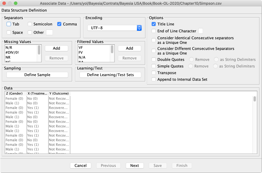
Given that the Associate Data Wizard mirrors the Data Import Wizard in most of its options, we omit to describe them here. We merely show the screens for reference as we click Next to progress through the wizard.
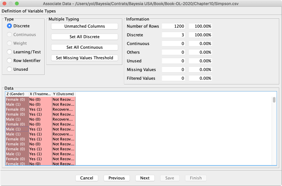
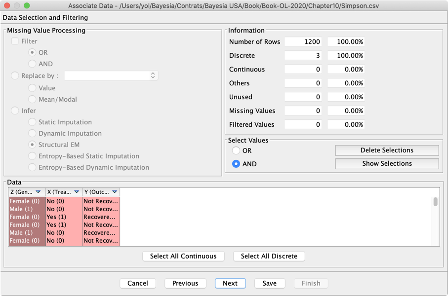
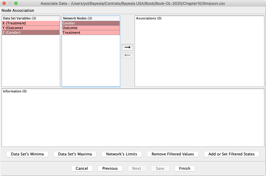
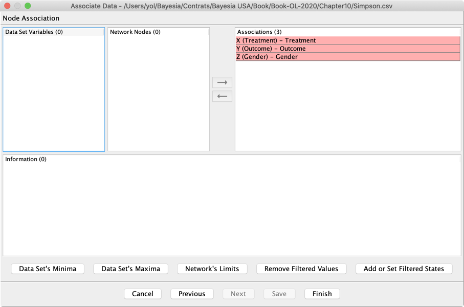
The last step shows how the variables in the dataset will be associated with the nodes of the network. If the column names in the dataset perfectly match the existing node names, BayesiaLab automatically creates an association. However, this is not the case in our example. Therefore, we have to manually define the association by iteratively selecting each Dataset Variable and Network Node, and then clicking on the right arrow.
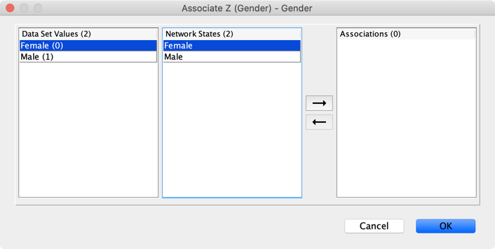
Upon clicking on the right arrow, BayesiaLab brings up a screen for defining the association between the values used in the dataset and the states of the node. Again, the state names of our nodes do not correspond exactly to the values used in the dataset. So we have to manually define the association by iteratively selecting each Dataset Value and Network State and then clicking on the right arrow.
Once this is done for all three variables, the Associate Data Wizard displays how the columns in the dataset are associated with the nodes of the network.
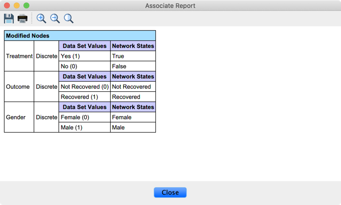
Upon clicking Finish, we are prompted whether we want to view the Associate Report.
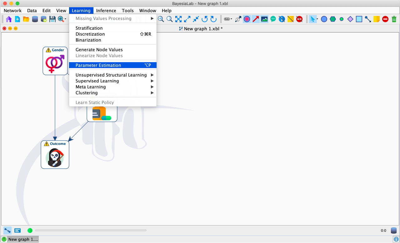
The Database icon in the lower right-hand corner of the main window indicates that our network now has a database associated with its structure. We now use this data to estimate the parameters of the network: Learning > Parameter Estimation.
Once the parameters are estimated, there are no longer any warning symbols tagged onto the nodes.
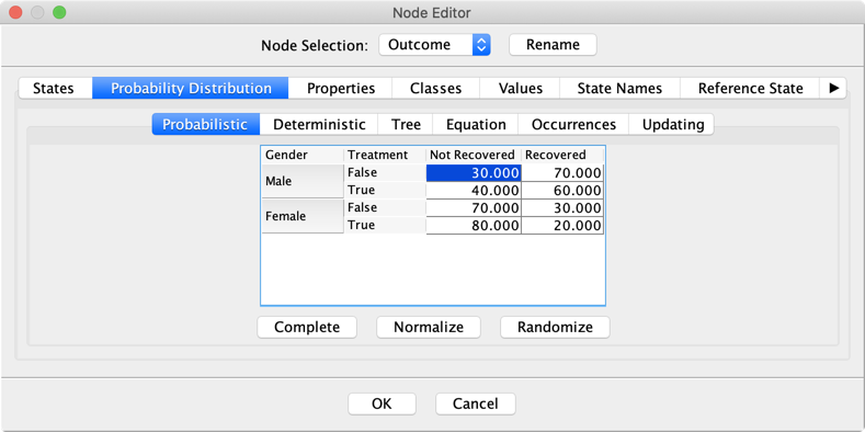
We now have a fully specified Bayesian network. By opening the Node Editor of Outcome, for instance, we see that the CPT is indeed filled with probabilities.
Upon clicking on the Occurrences tab, we can see the counts that were used by the Maximum Likelihood Estimation to derive these probabilities.

Path Analysis
Recall that distinguishing between causal and non-causal paths is crucial for the application of the Adjustment Criterion. BayesiaLab can help us review the paths that are present in the graph. Given that we already understand the paths, showing the formal path analysis with BayesiaLab is merely for reference.
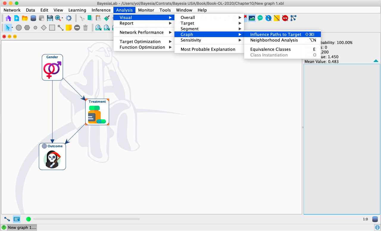
Once we define Outcome as Target Node and switch into the Validation Mode F5, we can examine all possible paths to the Target Node in this network. We select Treatment and then select Menu > Analysis > Visual > Graph > Influence Paths to Target.
Then, BayesiaLab displays a pop-up window with the Influence Paths report. Selecting any of the listed paths shows the corresponding arcs in the Graph Panel. Causal paths are shown in blue; non-causal paths are pink.
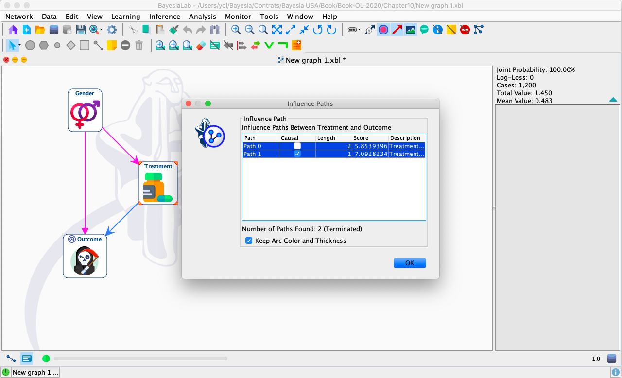
It is easy to see that this automated path analysis can be particularly helpful with more complex networks. In any case, the result confirms our previous manual path analysis, which means that we need to adjust for Gender to block the non-causal path between Treatment and Outcome.
Observational Inference
Before proceeding to the effect estimation, we bring up the Monitors of all three nodes and compare the probabilities reported by the network with the Aggregate and Gender-Specific Tables, which gave rise to the paradox.
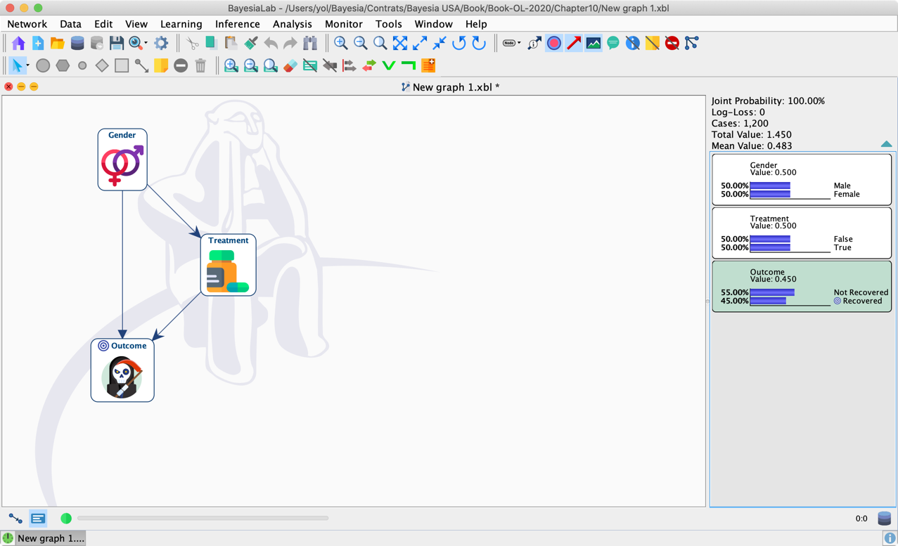
For instance, the screenshot below shows the prior distributions (left) and the posterior distributions (right) given the observation Treatment = True.
As expected, the target variable Outcome changes upon setting this evidence. However, Gender changes as well, even though we know that the treatment cannot possibly change the gender of a patient. What we observe here is a manifestation of the non-causal path: Treatment ← Gender → Outcome. These probabilities are obviously perfectly correct from the observational point of view: in the observed population of 1,200 individuals, three times as many men as women took the treatment.
Causal Inference
For causal inference, however, we need a network that computes all probabilities under an intervention scenario. As we learned, Graph Surgery transforms the original causal network representing the pre-intervention distribution into a new, mutilated network that yields the post-intervention distribution.
In BayesiaLab, Graph Surgery is automated. After right-clicking the Monitor of the node Treatment, we select Intervention from the Contextual Menu.
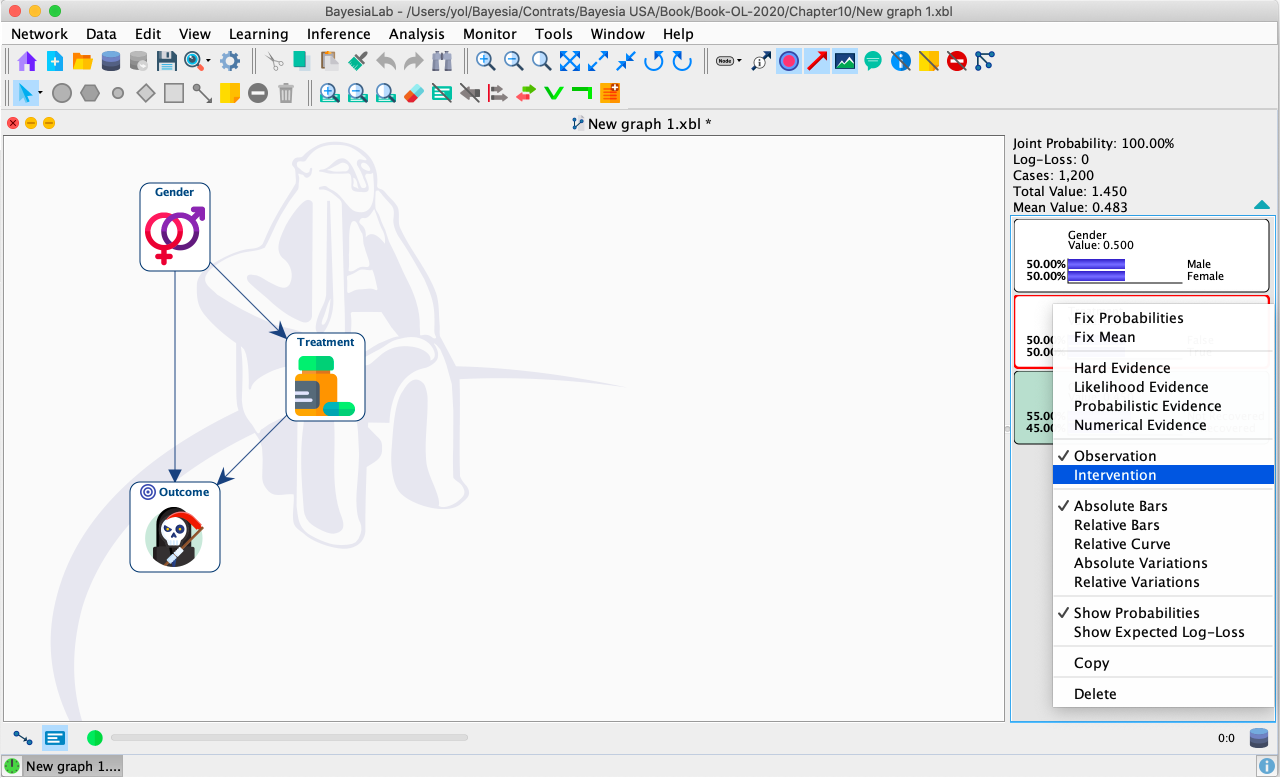
The activation of the Intervention Mode for this node is highlighted by the blue background of the Treatment’s Monitor and the arrow symbols (→) in the Treatment’s badge.
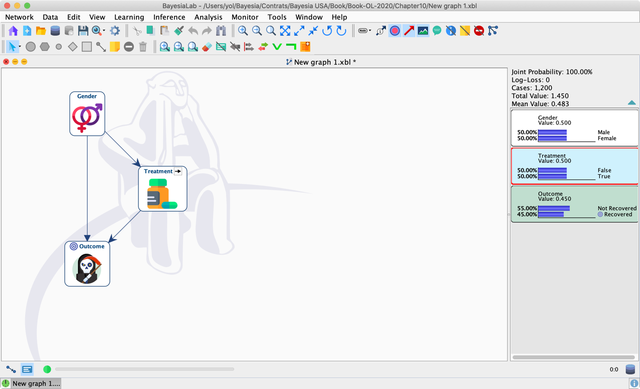
By double-clicking a state of Treatment, we now set an Intervention and no longer an Observation.
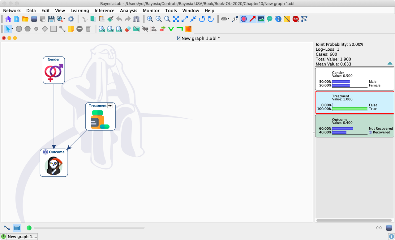
By intervening on Treatment, BayesiaLab applies Graph Surgery and removes the inbound arc into Treatment.
Recall the formula that computes the Average Causal Effect (ACE):
We can take it directly as a set of instructions and compare the probability of Outcome=Recovered under do(Treatment=False) and do(Treatment=True). Note that the distribution of Gender remains the same pre- and post-intervention.
Thus, we obtain an Average Causal Effect of −0.1, which agrees with what we previously computed with the Adjustment Formula.
