Information Gain (9.0)

Context

The Log-Loss LL(E) reflects the cost to process a particle E with a model, i.e. the number of bits that are needed to encode the particle E given the model. The lower the probability is, i.e. the more surprising a particle is given our model, the higher the log-loss is.

$\displaystyle LL(E) = - \log_2(P(E))$

where P(E) is the joint probability of the n-dimensional evidence E returned by the Bayesian network:

$\displaystyle P(E) = P({e_1},...,{e_n})$

The Information Gain is the difference between the cost to process a particle E with the fully unconnected network (the straw model S, where all nodes are marginally independent), and the cost with the current Bayesian network B:

$\displaystyle IG(E) = \log_2 \left( \frac{P(e_1, \dots, e_n)}{\prod_{i=1}^{n} P(e_i)} \right) = LL_S(E) - LL_B(E)$

Usage

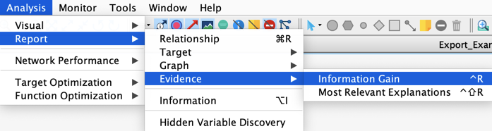
Select Menu > Analysis > Report > Evidence > Information Gain

History

This function, previously called Evidence Analysis Report, has been first updated in version 5.0.2.

Renamed Metrics: Local Information Gain

The metric used to compare the cost to represent the posterior probability of the 1-piece of hypothetical evidence h given the current set of evidence E and its prior probability is now called Local Information Gain instead of Information Gain.

$\displaystyle LIG(E, h) = \log_2 \left( \frac{P(h \mid E)}{P(h)} \right) = LL(h) - LL(h \mid E)$

Renamed Metrics: Hypothetical Information Gain

What would be the Information Gain if h, a 1-piece of evidence, were added to the current set of evidence E? This metric was called Bayes Factor in the previous releases.

$\displaystyle IG(E,h) = IG(E) + LIG(E,h)$

New Feature: Analysis of the Selected Nodes Only

As of version 9.0, the analysis can be carried out on the selected nodes only.

Example

Let’s use the network below with the following three pieces of evidence E:

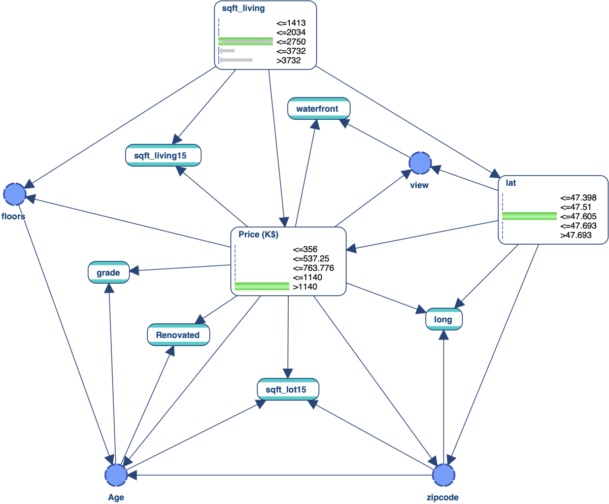
We select the nodes $\mathit{waterfront}$, $\mathit{view}$, $\mathit{Age}$, $\mathit{Renovated}$, and $\mathit{grade}$ and run the analysis on these five nodes only:

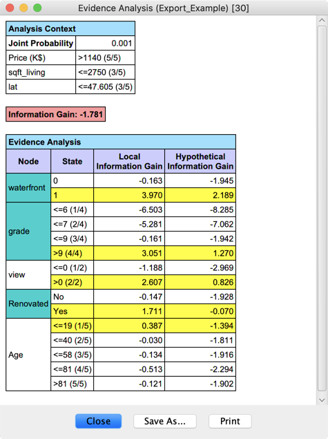
As we can see, the Information Gain of E with this network is negative (-1.781). A negative Information Gain is sometimes referrsed to a “conflict.”

However, if we were to add the evidence $\mathit{waterfront} = 1$, this would make the Information Gain of the new set of evidence positive (2.189). As such, this est of evidence is considered “consistent.”