Chapter 4: Knowledge Modeling and Probabilistic Reasoning

This chapter introduces a practical workflow for encoding expert knowledge and conducting omnidirectional probabilistic inference in the context of a real-world reasoning problem. While Chapter 1 outlined the general motivation for using Bayesian networks as an analytical framework, this chapter emphasizes their often overlooked relevance for modeling everyday reasoning. The example illustrates that what we perceive as common sense reasoning can, in fact, be quite complex. Yet representing such knowledge in a Bayesian network proves to be remarkably straightforward. Our goal is to show that reasoning with Bayesian networks can be as intuitive and accessible as performing calculations in a spreadsheet.

Background & Motivation

Complexity & Cognitive Challenges

Reasoning in complex environments presents significant cognitive challenges for humans. Uncertainty in our observations, or in the structure of the domain itself, further complicates the task. When such uncertainty obscures the underlying premises, it becomes particularly difficult to establish a shared reasoning framework among stakeholders.

No Data, No Analytics

If we had concrete data from the domain, it would be straightforward to develop a traditional analytical model for decision support. In practice, however, we often encounter fragmented datasets—or sometimes no data at all. In such cases, we must rely on the judgments of individuals who are familiar with the problem to varying degrees.

To an Analyst With Excel, Every Problem Looks Like Arithmetic

In the business world, spreadsheets are commonly used to model relationships among variables within a problem domain. When hard data are lacking, experts are often expected to provide assumptions in place of observations. This expert knowledge is typically encoded as single-point estimates and formulas. However, relying solely on fixed values and equations can oversimplify the complexity of the domain. First, it renders the variables and their relationships deterministic. Second, the structure of formulas, defined by a left-hand side and a right-hand side, restricts inference to a single direction.

Taking No Chances!

Since the cells and formulas in spreadsheets are deterministic and operate using single-point values, they are well-suited to encoding “hard” logic. However, they struggle with “soft” probabilistic knowledge, which inherently involves uncertainty. As a result, any uncertainty must be managed through workarounds such as testing multiple scenarios or using simulation add-ons.

It Is a One-Way Street!

However, the lack of omnidirectional inference may be the more fundamental limitation of spreadsheets. As soon as we create a formula linking two cells, e.g., $\mathit{B1} = \operatorname{function}(\mathit{A1})$, we preclude evaluation in the opposite direction, from $\mathit{B1}$ to $\mathit{A1}$.

Even assuming that $\mathit{A1}$ is the cause and $\mathit{B1}$ the effect, we can only use a spreadsheet for inference in the causal direction (i.e., simulation). Yet unidirectionality remains a concern even when the causal direction is known. For instance, if we can observe only the effect $\mathit{B1}$, we are unable to infer the cause $\mathit{A1}$—that is, we cannot perform diagnostic reasoning. This one-way structure is inherent to spreadsheet computations.

Bayesian Networks to the Rescue!

Bayesian networks are probabilistic by design and handle uncertainty natively. A Bayesian network model can work directly with probabilistic inputs and relationships, producing correctly computed probabilistic outputs. In contrast to traditional models and spreadsheets, which are typically expressed as $y = f(x)$, Bayesian networks do not require a strict distinction between independent and dependent variables. Instead, they represent the full joint probability distribution of the system under study. This representation enables omnidirectional inference, which is often essential for reasoning in complex problem domains—such as the one presented in this chapter.

Example: Where is My Bag?

While most examples in this book are drawn from formal research contexts, we introduce probabilistic reasoning with Bayesian networks through a more casual, everyday scenario. It reflects a familiar situation from daily life—one where a “common-sense” interpretation may seem more natural than a formal analytic approach. As we shall see, however, using formal methods to represent informal knowledge offers a powerful foundation for reasoning under uncertainty.

Did My Checked Luggage Make the Connection?

Most travelers will be familiar with the following scenario, or something like it: You’re flying from Singapore to Los Angeles with a connecting flight in Tokyo. Your flight from Singapore is significantly delayed, and you arrive in Tokyo with just enough time to make the connection. You sprint from Terminal 1, where you landed, to Terminal 2, where your flight to Los Angeles is already boarding as you reach the gate.

Click to Zoom

×

Problem #1

Out of breath, you check in with the gate agent, who tells you that your checked luggage from Singapore may or may not have made the connection. She apologetically says there’s only a 50/50 chance that your bag will arrive in Los Angeles.

After landing in Los Angeles, you head straight to baggage claim. Bags begin arriving steadily on the carousel. Five minutes go by, and you watch other passengers collect their luggage. You start to wonder: what are the chances that your bag will appear?

You reason that if your bag did make it onto the plane, it becomes more likely to show up as time passes. But you still don’t know whether it was ever loaded. Should you wait longer? Or is it time to get in line at the baggage office to file a claim? How should you update your expectations as the minutes tick by and your bag hasn’t yet appeared?

Problem #2

As you contemplate your next move, you see a colleague picking up his suitcase. As it turns out, your colleague was traveling on the very same itinerary as you, i.e., Singapore – Tokyo – Los Angeles. His luggage made it, so you conclude that you better wait at the carousel for the very last piece to be delivered. How does the observation of your colleague’s suitcase change your belief in the arrival of your bag? Does all that even matter? After all, the bag either made the connection or not. The fact that you now observe something after the fact cannot influence what happened earlier, right?

Knowledge Modeling for Problem #1

This problem domain can be explained by a causal Bayesian network, only using a few common-sense assumptions. We demonstrate how to combine different pieces of available — but uncertain — knowledge into a network model. Our objective is to calculate the correct degree of belief in the arrival of your luggage as a function of time and your own observations.

Per our narrative, we obtain the first piece of information from the gate agent in Tokyo who manages the departure to Los Angeles. She says there is a 50/50 chance that your bag is on the plane. More formally, we express this as:

$P(\mathit{Your\, Bag\, on\, Plane} = \mathrm{True}) = 0.5$

We encode this probabilistic knowledge in a Bayesian network by creating a node. In BayesiaLab, we click the Node Creation Mode icon and then point to the desired position on the Graph Panel.

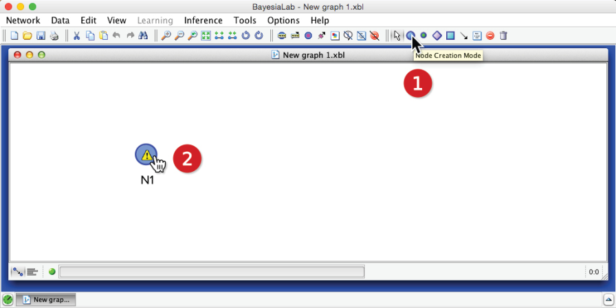
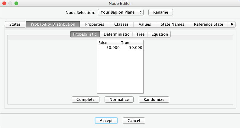
Once the node is in place, we update its name to $\mathit{Your\,Bag\,on\,Plane}$ by double-clicking the default name $\mathit{N1}$. Then, by double-clicking the node itself, we open BayesiaLab’s Node Editor. Under the tab Probability Distribution > Probabilistic, we define the probability that $\mathit{Your\,Bag\,on\,Plane}=\mathrm{True}$, which is 50%, as per the gate agent’s statement. Given that these probabilities do not depend on any other variables, we speak of marginal probabilities. Note that in BayesiaLab, probabilities are always expressed as percentages:

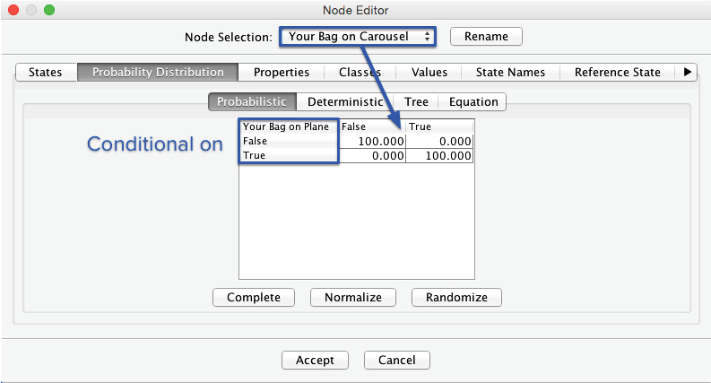
Assuming there is no other opportunity for losing luggage within the destination airport, your chance of ultimately receiving your bag should be identical to the probability of your bag being on the plane, i.e., on the flight segment to your final destination airport. More simply, if it is on the plane, then you will get it:

$P(\mathit{Your\, Bag\, on\, Carousel} = \mathrm{True} \bigm| \mathit{Bag\, on\, Plane} = \mathrm{True}) = 1$

$P(\mathit{Your\, Bag\, on\, Carousel} = \mathrm{False} \bigm\vert \mathit{Your\, Bag\, on\, Plane} = \mathrm{True}) = 0$

Conversely, the following must hold too:

$P(\mathit{Your\, Bag\, on\, Carousel} = \mathrm{False} \bigm| \mathit{Your\, Bag\, on\, Plane} = \mathrm{False}) = 1$

$P(\mathit{Your\, Bag\, on\, Carousel} = \mathrm{True} \bigm| \mathit{Your\, Bag\, on\, Plane} = \mathrm{False}) = 0$

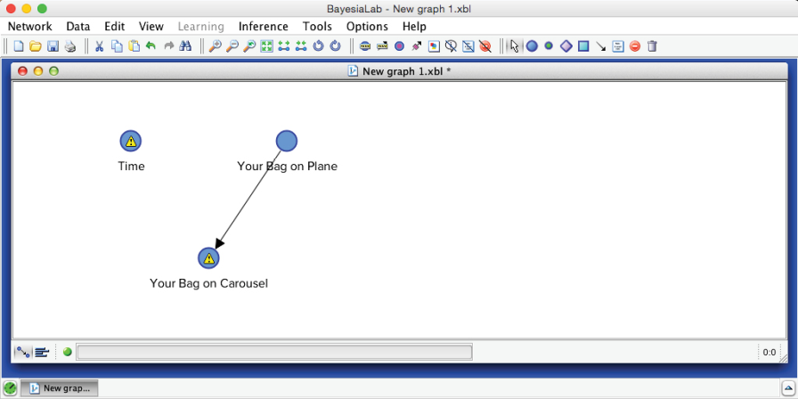
We now encode this knowledge into our network. We add a second node, $\mathit{Your\, Bag\, on\, Carousel}$, and then click the Arc Creation Mode icon . Next, we click and hold the cursor on $\mathit{Your\, Bag\, on\, Plane}$, drag the cursor to $\mathit{Your\, Bag\, on\, Carousel}$, and finally release. This produces a simple, manually specified Bayesian network:

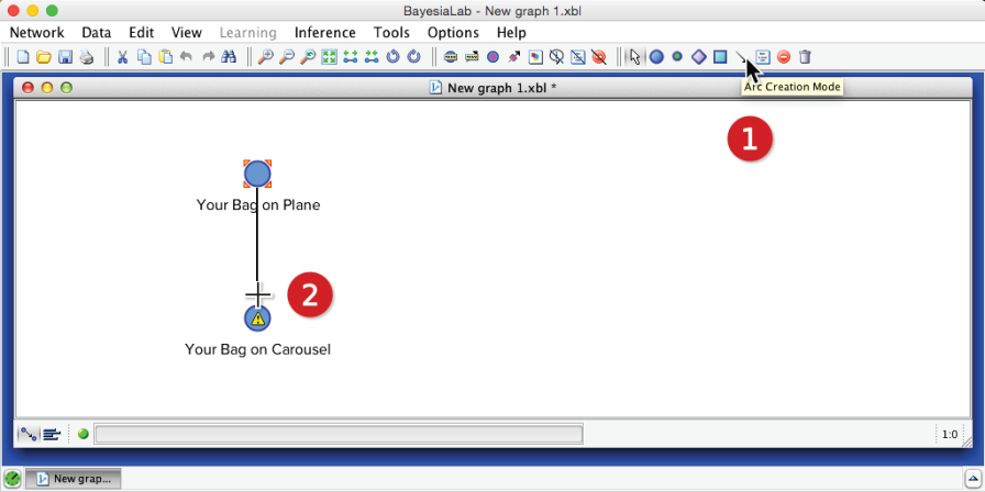
The yellow warning triangle indicates that probabilities need to be defined for the node $\mathit{Your\, Bag\, on\, Carousel}$. Unlike the previous instance, where we only had to enter marginal probabilities, we now need to define the probabilities of the states of the node $\mathit{Your\, Bag\, on\, Carousel}$ conditional on the states of $\mathit{Your\, Bag\, on\, Plane}$. In other words, we need to fill the Conditional Probability Table to quantify this parent-child relationship. We open the Node Editor and enter the values from the equations above.

Introduction of Time

Now we add another piece of contextual information that has not been mentioned yet in our story. From the baggage handler who monitors the carousel, you learn that 100 pieces of luggage in total were on your final flight segment, from the hub to the destination. After you wait for one minute, 10 bags have appeared on the carousel, and they keep coming out at a very steady rate. However, yours is not among the first ten that were delivered in the first minute. At the current rate, it would now take 9 more minutes for all bags to be delivered to the baggage carousel.

Given that your bag was not delivered in the first minute, what is your new expectation of ultimately getting your bag? How about after the second minute of waiting? Quite obviously, we need to introduce a time variable into our network. We create a new node $\mathit{Time}$ and define discrete time intervals [0,...,10] to serve as its states.

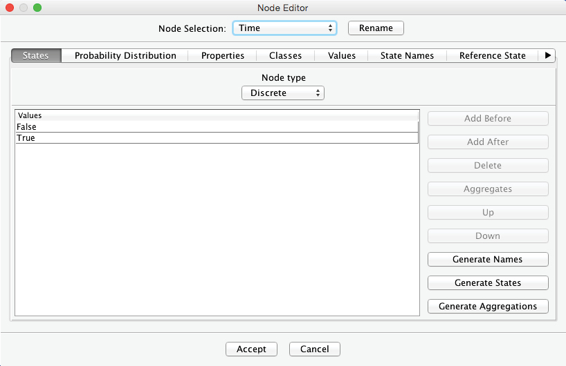
By default, all new nodes initially have two states, $\mathrm{True}$ and $\mathrm{False}$. We can see this by opening the Node Editor and selecting the States tab:

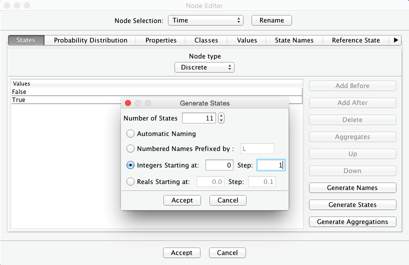
By clicking on the Generate States button, we create the states we need for our purposes. Here, we define 11 states, starting at 0 and increasing by 1 step:

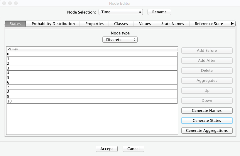
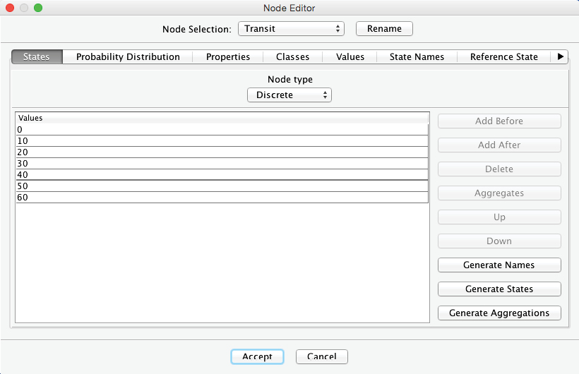
The Node Editor now shows the newly-generated states:

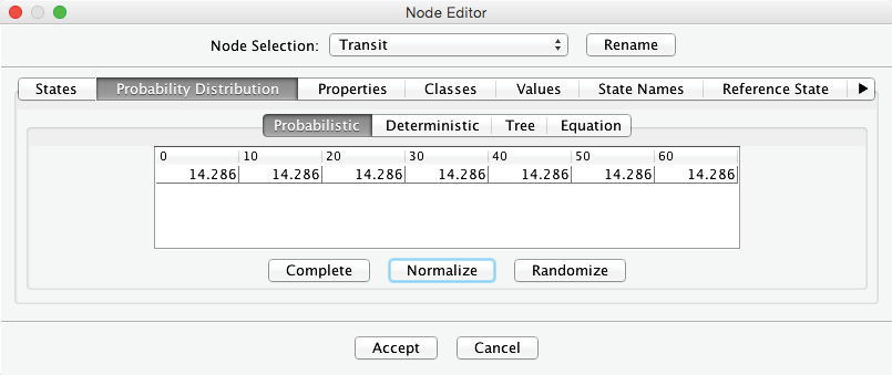
Beyond defining the states of $\mathit{Time}$, we also need to define their marginal probability distribution. For this, we select the tab Probability Distribution > Probabilistic. Naturally, no time interval is more probable than another one, so we should apply a uniform distribution across all states of $\mathit{Time}$. BayesiaLab provides a convenient shortcut for this purpose. Clicking the Normalize button places a uniform distribution across all cells, i.e., 9.091% per cell.

Once $\mathit{Time}$ is defined, we draw an arc from $\mathit{Time}$ to $\mathit{Your\, Bag\, on\, Carousel}$. By doing so, we introduce a causal relationship, stating that $\mathit{Time}$ influences the status of your bag.

The warning triangle once again indicates that we need to define further probabilities concerning $\mathit{Your\,Bag\,on\,Carousel}$. We open the Node Editor to enter these probabilities into the Conditional Probability Table:

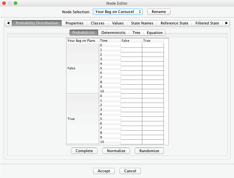
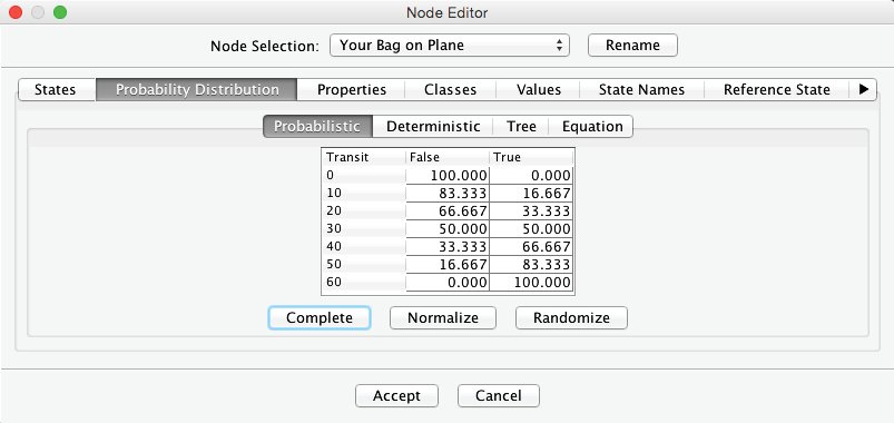
Note that the probabilities of the states $\mathrm{True}$ and $\mathrm{False}$ now depend on two-parent nodes. For the upper half of the table, it is still quite simple to establish the probabilities. If the bag is not on the plane, it will not appear on the baggage carousel under any circumstance, regardless of $\mathit{Time}$. Hence, we set $\mathrm{False}$ to 100 (%) for all rows in which $\mathit{Your\, Bag\, on\, Plane} = \mathrm{False}$.

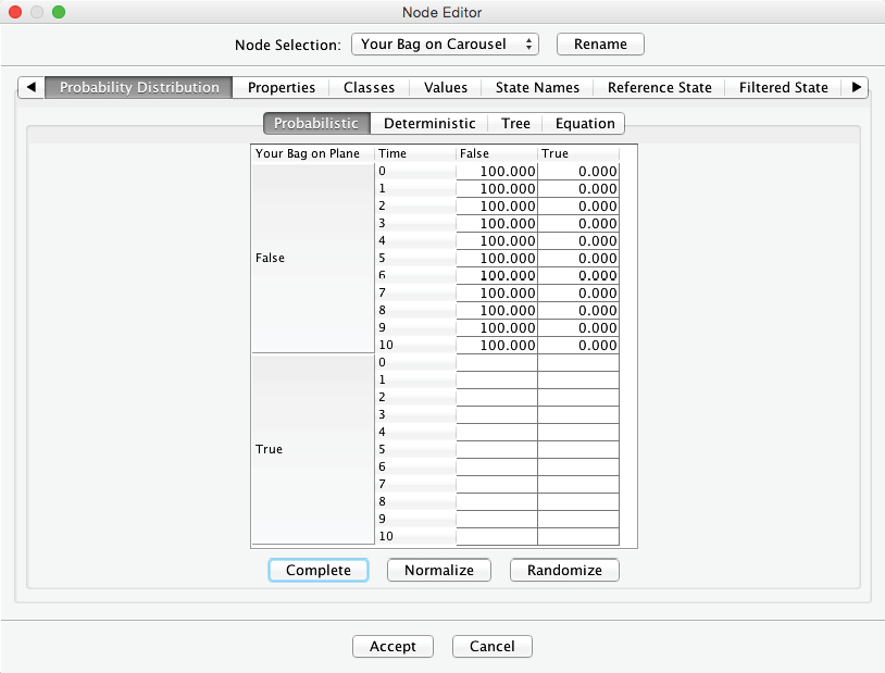
However, given that $\mathit{Your\, Bag\, on\, Plane} = \mathrm{True}$, the probability of seeing it on the carousel depends on the time elapsed. Now, what is the probability of seeing your bag at each time step? Assuming that all luggage is shuffled extensively through the loading and unloading processes, there is a uniform probability distribution that the bag is anywhere in the pile of luggage to be delivered to the carousel. As a result, there is a 10% chance that your bag is delivered in the first minute, i.e., within the first batch of 10 out of 100 luggage pieces. Over a period of two minutes, there is a 20% probability that the bag arrives, and so on. Only when the last batch of 10 bags remains undelivered, we can be certain that your bag is in the final batch, i.e. there is a 100% probability of the state $\mathrm{True}$ in the tenth minute. We can now fill out the Conditional Probability Table in the Node Editor with these values. Note that we only need to enter the values in the $\mathrm{True}$ column and then highlight the remaining empty cells. Clicking Complete prompts BayesiaLab to automatically fill in the $\mathrm{False}$ column to achieve a row sum of 100%:

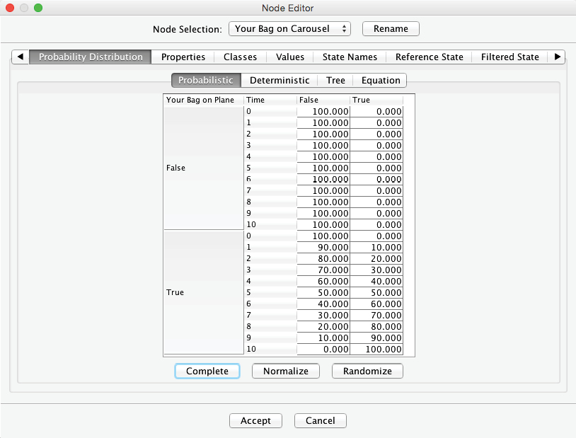
Now we have a fully specified Bayesian network, which we can evaluate immediately.

Evidential Reasoning for Problem #1

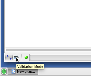
BayesiaLab’s Validation Mode F5 provides the tools for using the Bayesian network we built for omnidirectional inference. We switch to the Validation Mode F5 via the corresponding , in the lower left-hand corner of the main window, or via the keyboard shortcut F5:

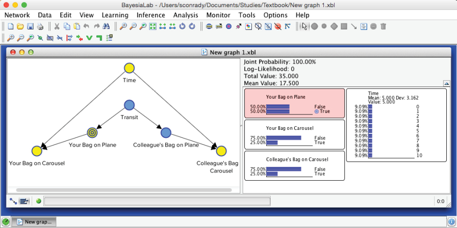
Upon switching to this mode, we double-click on all three nodes to bring up their associated Monitors, which show the nodes’ current marginal probability distributions. We find these Monitors inside the Monitor Panel on the right-hand side of the Graph Window:

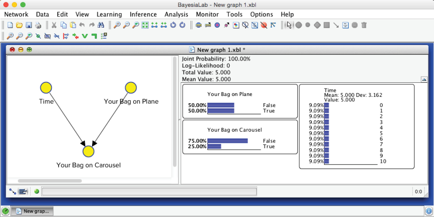
Inference Tasks

If we filled the Conditional Probability Table correctly, we should now be able to validate at least the trivial cases straight away, e.g. for $\mathit{Your\, Bag\, on\, Plane} = \mathrm{False}$.

Inference from Cause to Effect: $\mathit{Your\, Bag\, on\, Plane} = \mathrm{False}$

We perform inference by setting such evidence via the corresponding Monitor in the Monitor Panel. We double-click the bar that represents the State $\mathrm{False}$:

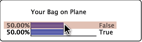
The setting of the evidence turns the node and the corresponding bar in the Monitor green:

The Monitor for $\mathit{Your\, Bag\, on\, Carousel}$ shows the result. The small gray arrows overlaid on top of the horizontal bars furthermore indicate how the probabilities have changed by setting this most recent piece of evidence:

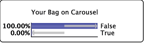
Indeed, your bag could not possibly be on the carousel because it was not on the plane in the first place. The inference we performed here is indeed trivial, but it is reassuring to see that the Bayesian network properly “plays back” the knowledge we entered earlier.

Omnidirectional Inference: $\mathit{Your\, Bag\, on\, Carousel} = \mathrm{False}, \mathit{Time} = 1$

The next question, however, typically goes beyond our intuitive reasoning capabilities. We wish to infer the probability that your bag made it onto the plane, given that we are now in minute 1, and the bag has not yet appeared on the carousel. This inference is tricky because we now have to reason along multiple paths in our network.

Diagnostic Reasoning

The first path is from $\mathit{Your\, Bag\, on\, Carousel}$ to $\mathit{Your\, Bag\, on\, Plane}$. This type of reasoning from effect to cause is more commonly known as diagnosis. More formally, we can write:

$P(\mathit{Your\, Bag\, on\, Plane} = \mathrm{True} \bigm| \mathit{Your\, Bag\, on\, Carousel} = \mathrm{False})$

Inter-Causal Reasoning

The second reasoning path is from $\mathit{Time}$ via $\mathit{Your\,Bag\,on\,Carousel}$ to $\mathit{Your\,Bag\,on\,Plane}$. Once we condition on $\mathit{Your\,Bag\,on\,Carousel}$, i.e. by observing the value, we open this path, and information can flow from one cause, $Time$, via the common effect, $\mathit{Your\,Bag\,on\,Carousel}$, to the other cause, $\mathit{Your\,Bag\,on\,Plane}$. Hence, we speak of “inter-causal reasoning” in this context. The specific computation task is:

$P(\mathit{Your\,Bag\,on\,Plane}=\mathrm{True} \bigm| \mathit{Your\,Bag\,on\,Carousel} = \mathrm{False},\mathit{Time} = 1)$

Bayesian Networks as Inference Engine

How do we go about computing this probability? We do not attempt to perform this computation ourselves. Rather, we rely on the Bayesian network we built and BayesiaLab’s exact inference algorithms. However, before we can perform this inference computation, we need to remove the previous piece of evidence, i.e. $\mathit{Your\,Bag\,on\,Plane}=\mathrm{True}$. We do this by right-clicking the relevant node and then selecting Remove Evidence from the Monitor Contextual Menu. Alternatively, we can remove all evidence by clicking the Remove All Observations icon .

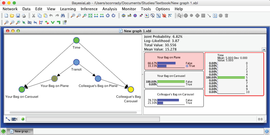
Then, we set the new observations via the Monitors in the Monitor Panel. The inference computation then happens automatically.

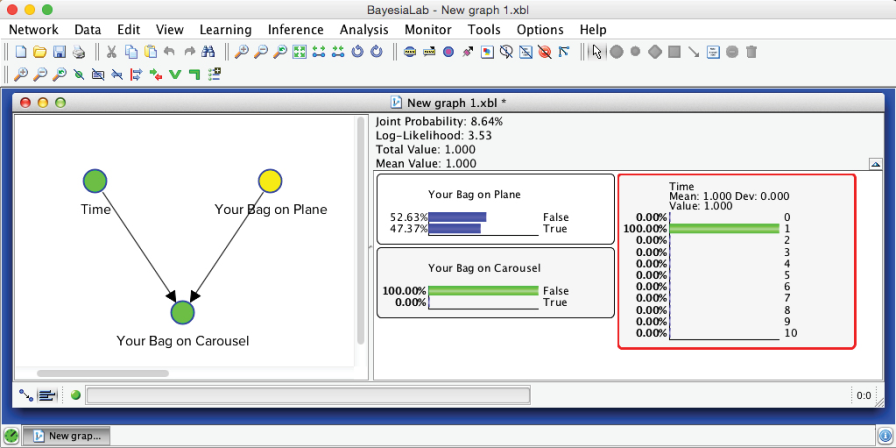
Given that you do not see your bag in the first minute, the probability that your bag made it onto the plane is now no longer at the marginal level of 50% but is reduced to 47.37%.

Inference as a Function of Time

Continuing with this example, how about if the bag has not shown up in the second minute, in the third minute, etc.? We can use one of BayesiaLab’s built-in visualization functions to analyze this automatically. To prepare the network for this type of analysis, we first need to set a Target Node, which, in our case, is $\mathit{Your\,Bag\,on\,Plane}$. Upon right-clicking this node, we select Set as Target Node. Alternatively, we can double-click the node, or one of its states in the corresponding Monitor, while holding T.

Upon setting the Target Node, $\mathit{Your\, Bag\, on\, Plane}$ is marked with a bullseye symbol . Also, the corresponding Monitor is now highlighted in red. Before we continue, however, we need to remove the evidence from the Monitor of $\mathit{Time}$. We do so by right-clicking the Monitor and selecting Remove Evidence from the Monitor Context Menu.

Then, we select Menu > Analysis > Visual > Target > Target Posterior > Histograms.

The resulting graph shows the probabilities of receiving your bag as a function of the discrete time steps. To see the progression of the $\mathrm{True}$ state, we select the corresponding tab at the top of the window.

Knowledge Modeling for Problem #2

Continuing with our narrative, you now notice a colleague of yours in the baggage claim area. As it turns out, your colleague was traveling on the same itinerary as you, i.e., Singapore – Tokyo – Los Angeles, so he had to make the same tight connection. Unlike you, he has already retrieved his bag from the carousel. You assume that his luggage being on the airplane is not independent of your luggage being on the same plane, so you take this as a positive sign. How do we formally integrate this assumption into our existing network?

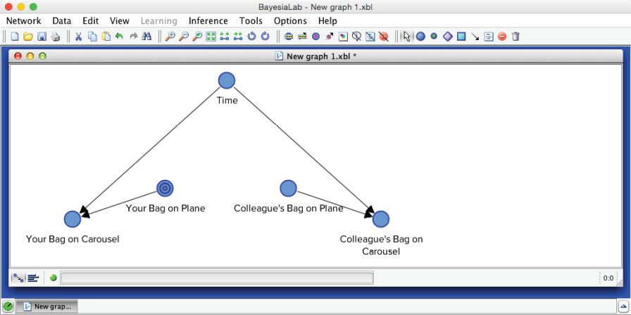
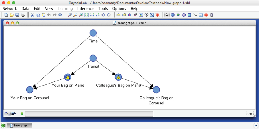
To encode any new knowledge, we first need to switch back to the Modeling Mode F4. Then, we duplicate the existing nodes $\mathit{Your\, Bag\, on\, Plane}$ and $\mathit{Your\, Bag\, on\, Carousel}$ by copying and pasting them into the same Graph Panel using the common shortcuts, Ctrl+C and Ctrl+V.

In the copy process, BayesiaLab prompts us for a Copy Format, which would only be relevant if we intended to paste the selected portion of the network into another application, such as PowerPoint. As we paste the copied nodes into the same Graph Panel, the format does not matter.

Upon pasting, by default, the new nodes have the same names as the original ones plus the suffix “[1]”.

Next, we reposition the nodes on the Graph Panel and rename them to show that the new nodes relate to your colleague’s situation, rather than yours. To rename the nodes we double-click the Node Names and overwrite the existing label.

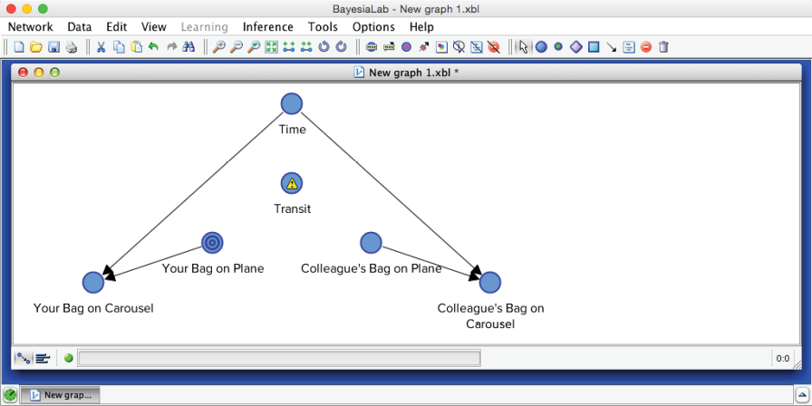
The next assumption is that your colleague’s bag is subject to exactly the same forces as your luggage. More specifically, the successful transfer of your and his luggage is a function of how many bags could be processed in Tokyo given the limited transfer time. To model this, we introduce a new node and name it $Transit$.

We create seven states of ten-minute intervals for this node, which reflect the amount of time available for the transfer, i.e., from 0 to 60 minutes.

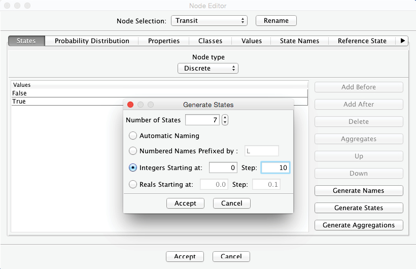
Furthermore, we set the probability distribution for $\mathit{Transit}$. To keep the example simple, we apply a uniform distribution using the Normalize button.

Now that the $\mathit{Transit}$ node is defined, we can draw the arcs connecting it to $\mathit{Your\,Bag\,on\,Plane}$ and $\mathit{Colleague’s\,Bag\,on\,Plane}$.

The yellow warning triangles indicate that the Conditional Probability Tables of $\mathit{Your\,Bag\,on\,Plane}$ and $\mathit{Colleague’s\,Bag\,on\,Plane}$ have yet to be filled. Thus, we need to open the Node Editor and set these probabilities. We will assume that the probability of your bag making the connection is 0% given a $\mathit{Transit}$ time of 0 minutes and 100% with a $\mathit{Transit}$ time of 60 minutes. Between those values, the probability of a successful transfer increases linearly with time.

The very same function also applies to your colleague’s bag, so we enter the same conditional probabilities for the node $\mathit{Colleague’s\,Bag\,on\,Plane}$ by copying and pasting the previously entered table.

Evidential Reasoning for Problem #2

Now that the probabilities are defined, we switch to the Validation Mode F5; our updated Bayesian network is ready for inference again.

We simulate a new scenario to test this new network. For instance, we move to the fifth minute and set evidence that your bag has not yet arrived.

Given these observations, the probability of $\mathit{Your\,Bag\,on\,Plane}=\mathrm{True}$ is now 33.33%. Interestingly, the probability of $\mathit{Colleague’s\,Bag\,on\,Plane}$ has also changed. As evidence propagates omnidirectionally through the network, our two observed nodes do indeed influence $\mathit{Colleague’s\,Bag\,on\,Plane}$. A further iteration of the scenario in our story is that we observe $\mathit{Colleague’s\,Bag\,on\,Carousel=True}$, also in the fifth minute.

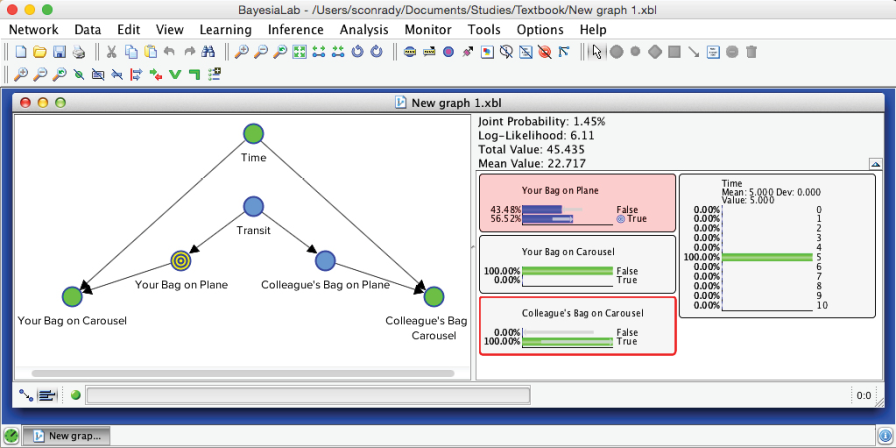
Given the observation of $Colleague’s\,Bag\,on\,Carousel$, even though we have not yet seen $\mathit{Your\,Bag\,on\,Carousel}$, the probability of $\mathit{Your\,Bag\,on\,Plane}$ increases to 56.52%. Indeed, this observation should change your expectation quite a bit. The small gray arrows on the blue bars inside the Monitor for $\mathit{Your\,Bag\,on\,Plane}$ indicate the impact of this observation.

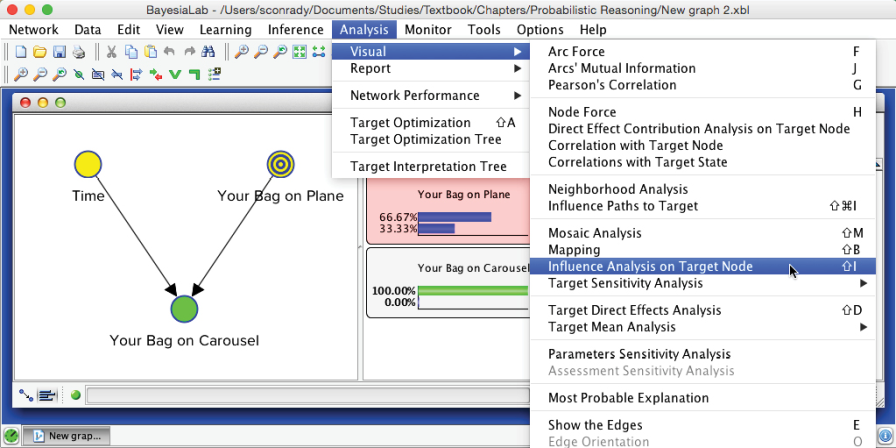
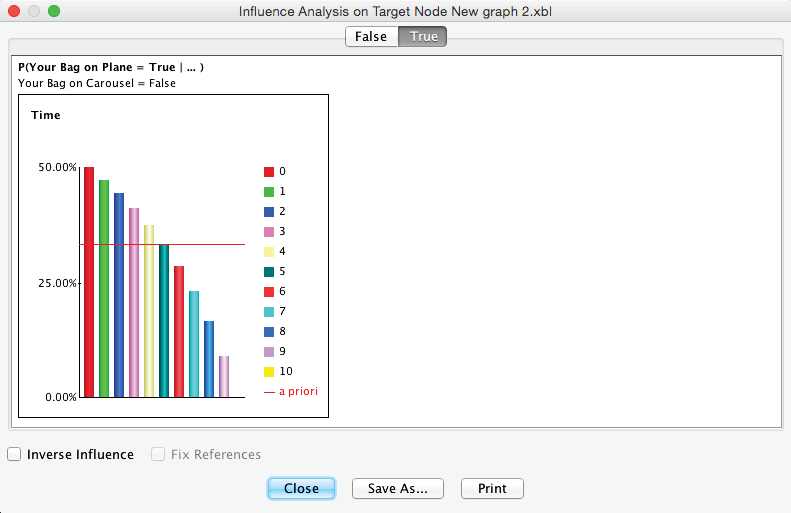
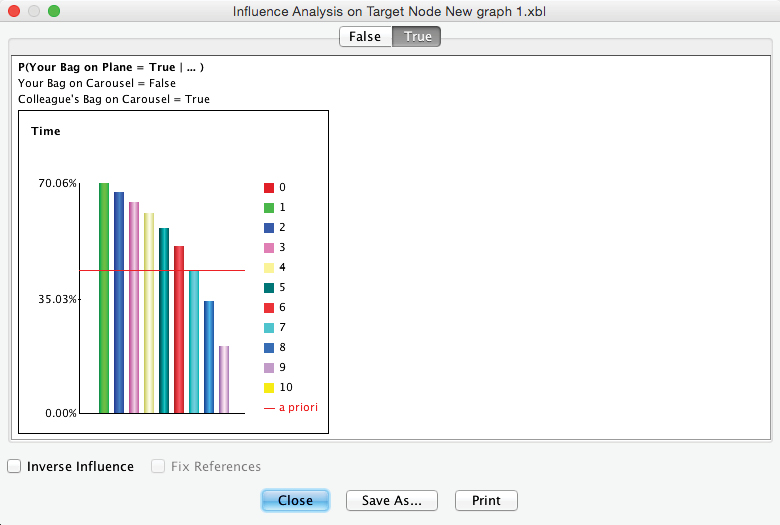
After removing the evidence from the $Time$ Monitor, we can perform Influence Analysis on Target again in order to see the probability of $\mathit{Your\,Bag\,on\,Plane}=\mathrm{True}$ as a function of $\mathit{Time}$, given $\mathit{Your\,Bag\, on\,Carousel}=\mathrm{False}$ and $\mathit{Colleague’s\,Bag\,on,Carousel}=\mathrm{True}$. To focus our analysis on $Time$ alone, we select the $Time$ node and then select Analysis > Visual > Influence Analysis on Target.

As before, we select the $\mathrm{True}$ tab in the resulting window to see the evolution of probabilities given $\mathit{Time}$.

Summary

This chapter provided a brief introduction to knowledge modeling and evidential reasoning with Bayesian networks in BayesiaLab. Bayesian networks can formally encode available knowledge, deal with uncertainties, and perform omnidirectional inference. As a result, we can properly reason about a problem domain despite many unknowns.