Step 2: Variable Clustering
BayesiaLab’s Variable Clustering is a hierarchical agglomerative clustering algorithm that uses Arc Force (i.e., the Kullback-Leibler Divergence) for computing the distance between nodes.
At the start of Variable Clustering, each manifest variable is treated as a distinct cluster. The clustering algorithm proceeds iteratively by merging the “closest” clusters into a new cluster. Two criteria are used for determining the number of clusters:
- Stop Threshold: a minimum Arc Force value below which clusters are not merged (a kind of significance threshold).
- Maximum Cluster Size: the maximum number of variables per cluster.
These criteria can be set via Menus > Window > Preferences > Learning > Variable Clustering:
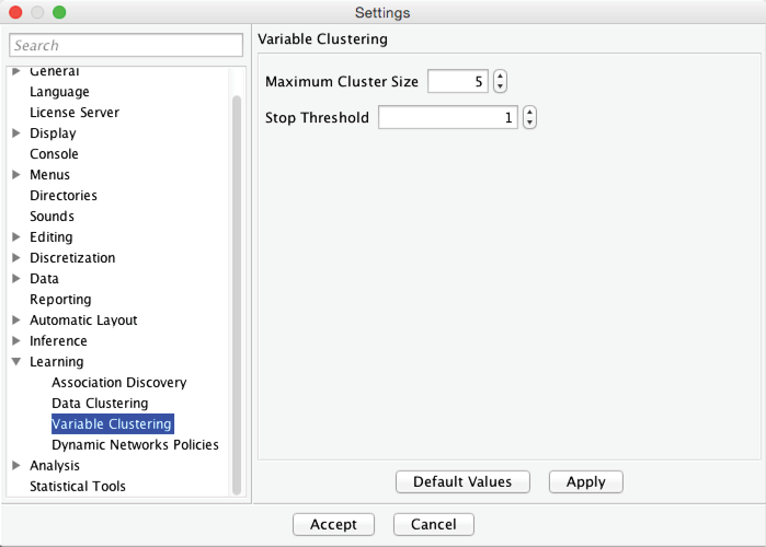
We do not advise changing the Stop Threshold, but Maximum Cluster Size is more subjective. For building PSEMs, we recommend a value between 5 and 7, for reasons that will become clear when we show how latent variables are generated. If, however, the goal of Variable Clustering is dimensionality reduction, we suggest increasing the Maximum Cluster Size to a much higher value, thus effectively eliminating it as a constraint.
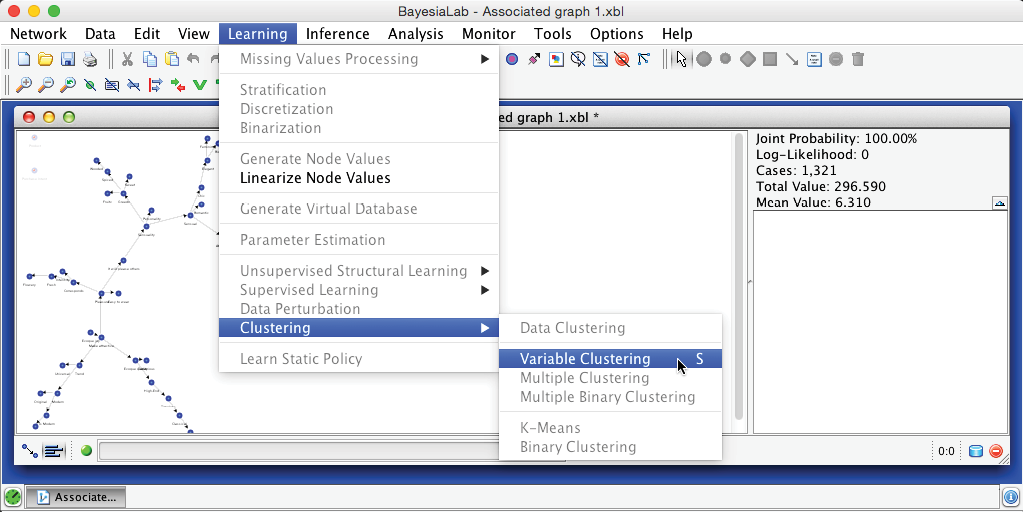
The Variable Clustering algorithm can be started via Main Menus > Learning > Clustering > Variable Clustering or by using the shortcut S.
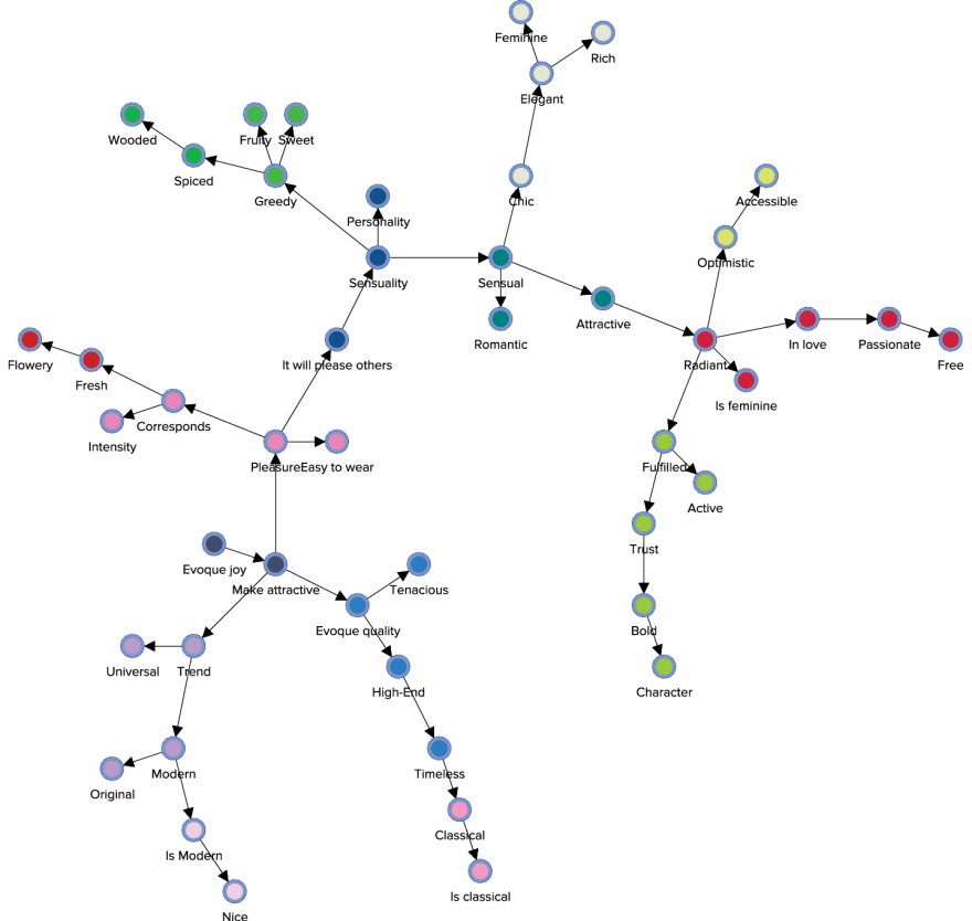
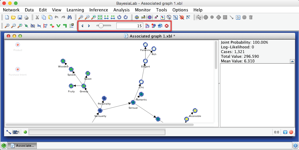
In this example, BayesiaLab identified 15 clusters, and each node is now color-coded according to its cluster membership. The following image shows the standalone graph, outside the BayesiaLab window, for better legibility.
BayesiaLab offers several tools for examining and editing the proposed cluster structure. They are accessible from an extended menu bar (highlighted in the screenshot below).
Dendrogram
The Dendrogram allows us to review the linkage of nodes within variable clusters. It can be activated via the corresponding icon in the extended menu. The lengths of the branches in the Dendrogram are proportional to the Arc Force between clusters.
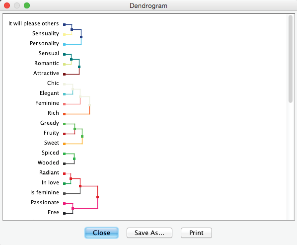
Also, the Dendrogram can be copied directly as a vector or bitmap graphic by right-clicking on it. Alternatively, it can be exported in various formats via the Save As… button. As such, it can be imported into documents and presentations. This ability to copy and paste graphics applies to most graphs, plots, and charts in BayesiaLab.

Cluster Mapping
Mapping offers an intuitive approach to examining the just-discovered cluster structure as an alternative to Dendrogram. It can be activated via the Mapping button in the menu bar.
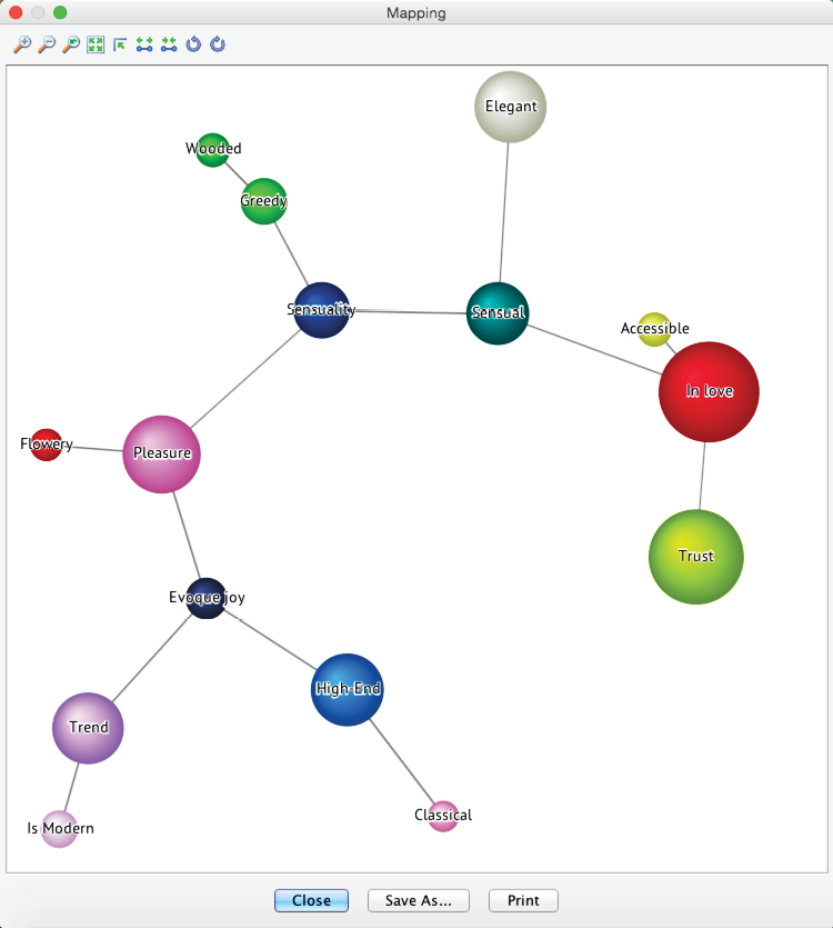
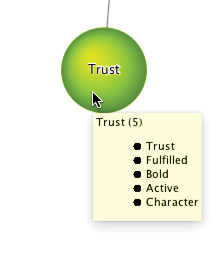
By hovering over any cluster “bubbles” with the cursor, BayesiaLab displays a list of all manifest nodes connected to that particular cluster. Each list of manifest variables is sorted according to the intra-cluster Node Force. This also explains the names displayed on the clusters. By default, each cluster takes on the name of the strongest manifest variable.
Number of Clusters
As explained earlier, BayesiaLab uses two criteria to determine the default number of clusters. We can change this number via the selector in the menu bar.

The Dendrogram and the Mapping view respond dynamically to any changes to the number of clusters.
Cluster Validation
The result of the Variable Clustering algorithm is purely descriptive. Once the question regarding the number of clusters is settled, we need to formally confirm our choice by clicking the Validate Clustering button in the toolbar. Only then can we trigger the creation of one Class per Cluster. At that time, all nodes become associated with unique Classes named , with representing the identifier of the factor. Additionally, we are prompted to confirm that we wish to keep the node colors generated during clustering.
The Clusters are now saved, and the color-coding is formally associated with the nodes. A Clustering Report provides a formal summary of the new Factors and their associated Manifest variables.
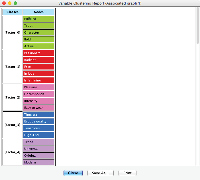
Note that we use the following terms interchangeably: “derived concept,” “unobserved latent variable,” “hidden cause,” and “extracted factor.”
The Classes icon in the lower right-hand corner of the window confirms that Classes have been created corresponding to the Factors. This concludes Step 2, and we formally close Variable Clustering via the stop icon on the extended toolbar.
Editing Factors
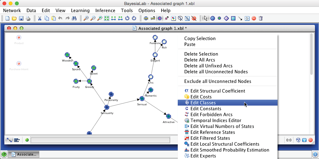
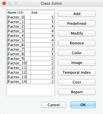
Beyond our choice with regard to the number of Clusters, we also have the option of using our domain knowledge to modify which Manifest Nodes belong to specific Factors. This can be done by right-clicking on the Graph Panel and selecting Edit Classes, and then Modify from the Contextual Menu. Alternatively, we can click the Classes icon . In our example, however, we show the Class Editor just for reference, as we keep all the original variable assignments in place.
Cluster Cross-Validation
We now examine the robustness of the identified factors, i.e., how these factors respond to changes in sampling. This is particularly important for studies that are regularly repeated with new data, e.g., annual customer satisfaction surveys. Inevitably, survey samples are going to be different between the years. As a result, machine learning will probably discover somewhat different structures each time and, therefore, identify different clusters of nodes. Therefore, it is important to distinguish between a sampling artifact and a substantive change in the joint probability distribution. In the context of our example, the latter would reveal a structural change in consumer behavior.
We start the validation process via Menus > Tools > Resampling > Variable Clustering > Data Perturbation.
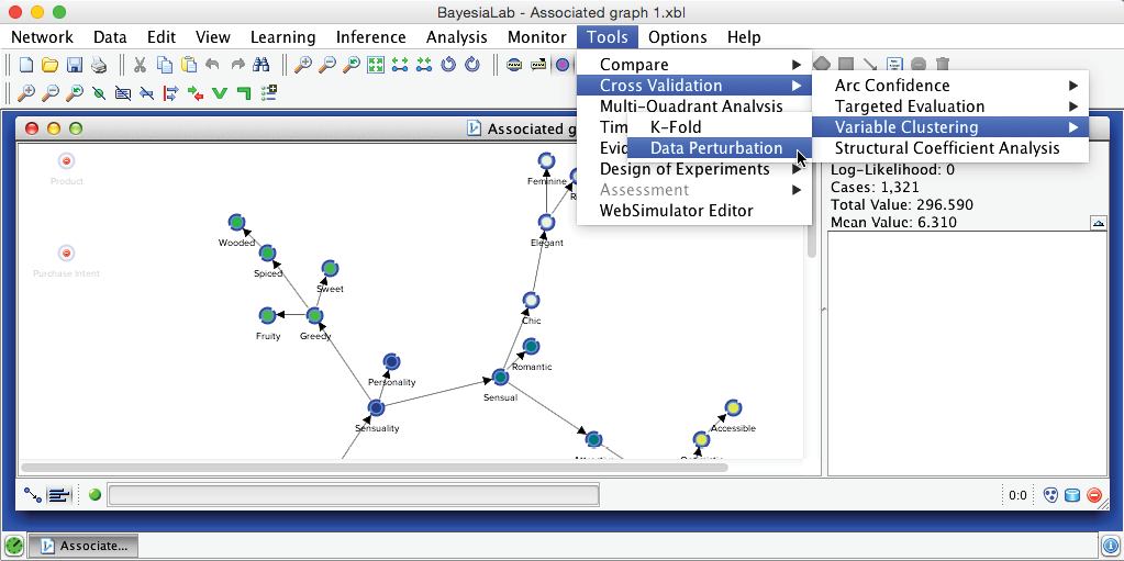
This brings up the dialogue box shown below.
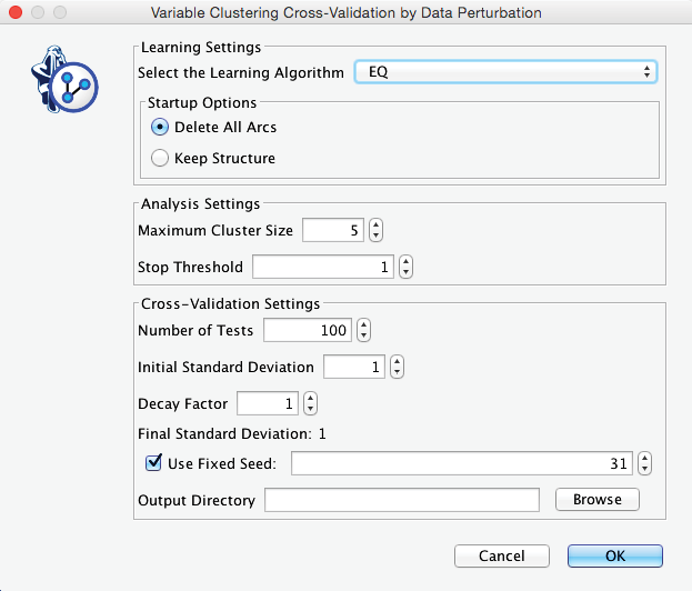
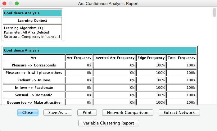
These settings specify that BayesiaLab will learn 100 networks with EQ and perform Variable Clustering on each of them, all while maintaining the constraint of a maximum of 5 nodes per cluster without any attenuation of the perturbation. Upon completion, we obtain a report panel, from which we initially select Variable Clustering Report.
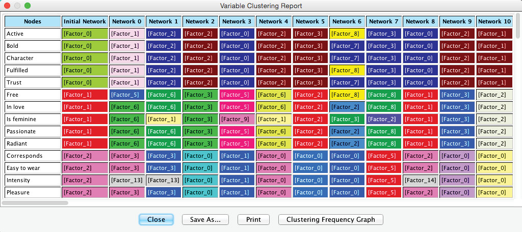
The Variable Clustering Report consists primarily of two large tables. The first table in the report shows the cluster membership of each node in each network (only the first 12 columns are shown). Here, thanks to the colors, we can easily detect whether nodes remain clustered together between iterations or whether they “break up.”
The second table shows how frequently individual nodes are clustered together.
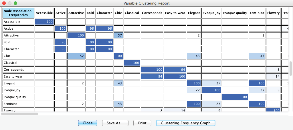
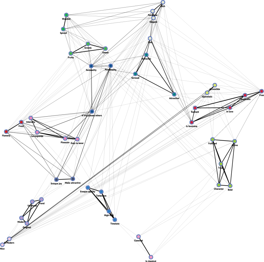
Clicking the Clustering Frequency Graph provides yet another visualization of the clustering patterns. The thickness of the lines is proportional to the frequency of nodes being in the same Cluster. Equally important for interpretation is the absence of lines between nodes. For instance, the absence of a line between and Modern says that they have never been clustered together in any of the 100 samples. If they were to cluster together in a future iteration with new survey data, it would probably reflect a structural change in the market rather than a data sampling artifact.