Inference: Automatic Evidence-Setting
Context
- Early in this chapter, we used the Augmented Markov Blanket algorithm to machine-learn a predictive model for classifying cell samples.
- Subsequently, we optimized the model with the Structural Coefficient Analysis workflow.
- We can now use the validated model for analysis and inference.
- In this and the next two sections of this chapter, we look at different ways of performing inference:
- Automatic-Evidence Setting
- Adaptive Questionnaire
- Target Interpretation Tree
Validation Mode
For all types of inference with a Bayesian network model, we need to switch to Validation Mode F5.
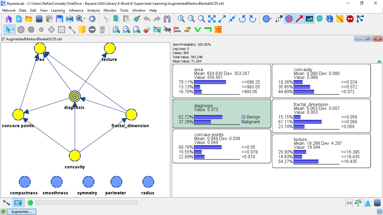
Before proceeding to Automatic Evidence-Setting, we bring up all the Monitors connected to the Target Node in the Monitor Panel.

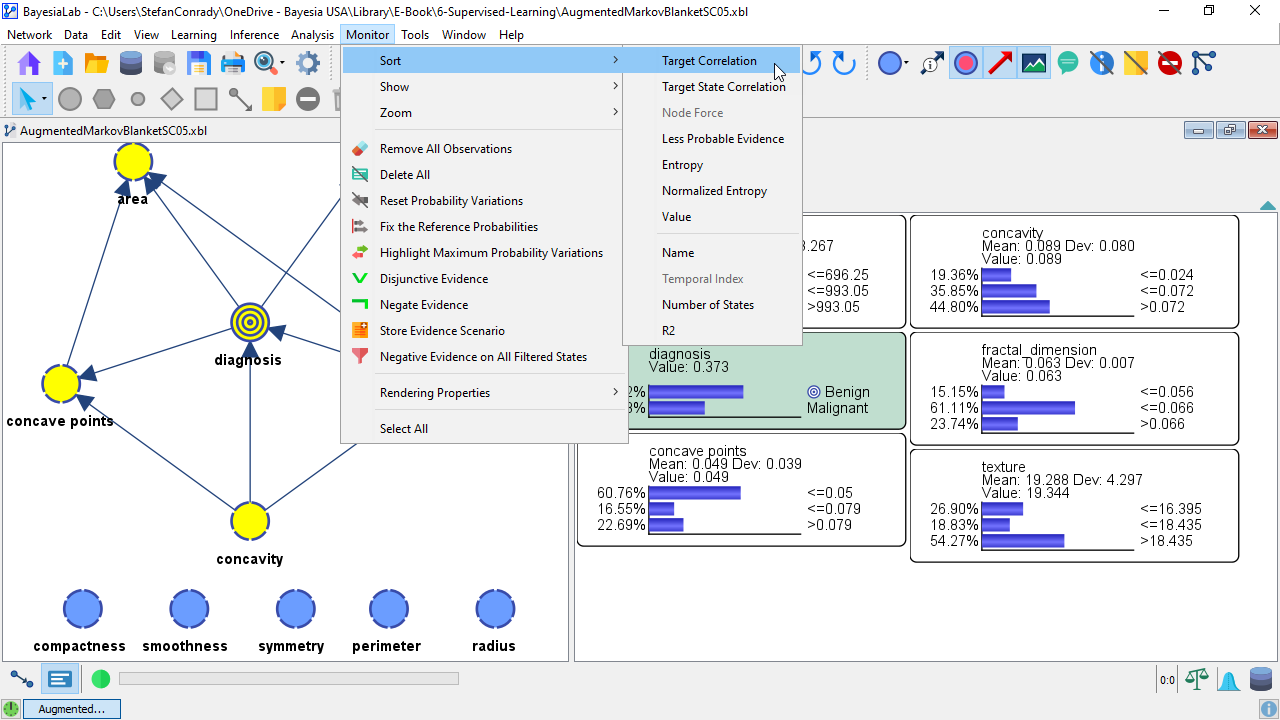
Since we have a Target Node, we can right-click inside the Monitor Panel to select Sort > Target Correlation from the Monitor Panel Context Menu.
Alternatively, we can do the same via Menu > Monitor > Sort > Target Correlation.

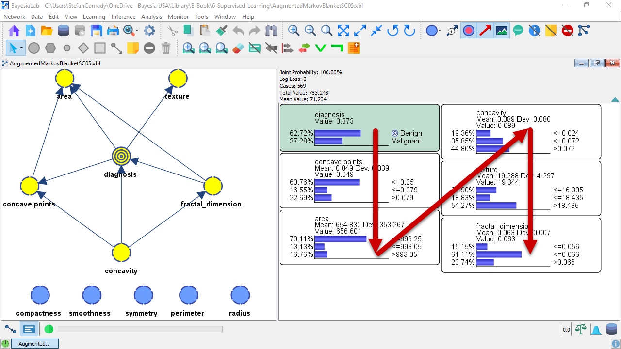
The Monitor of the Target Node is placed first in the Monitor Panel, followed by the other Monitors according to their “correlation” with the Target Node, from highest to lowest.
Note that we use “correlation” not literally in this context. Rather, the sort order of the Monitors is determined by Mutual Information.

Automatic Evidence Setting (Interactive Inference)
Given that we have a predictive model in place, we can use BayesiaLab to review its individual predictions record by record.
This feature is called Automatic Evidence-Setting, which can be accessed here: Menu > Inference > Automatic Evidence-Setting.
In earlier releases of BayesiaLab, this function was called Interactive Inference.
As an extension of the Main Menu, a Navigation Bar and its record selectors allow us to scroll through all records in the dataset.
Record #0
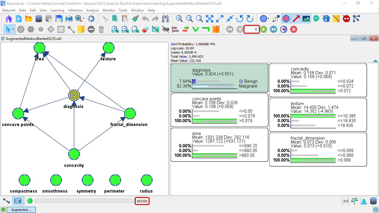
The first record in the dataset is displayed in the screenshot below as record #0.

Additionally, the Row Identifier, 842302, is displayed in the Status Bar to the right of the Progress Bar at the bottom of the Graph Window.
The Monitors display the values of the variables in that record, i.e., the set of evidence or observations.
Given these observations, the model predicts a 92.36% probability that the diagnosis is malignant (the Monitor of the Target Node features a green background).
With such a high probability, the prediction diagnosis=malignant is the rational prediction.
As it turns out, it is indeed the correct prediction for record #0 (Row Identifier 842302). The actual value recorded in the dataset is represented by a light blue bar, meaning diagnosis=malignant was the ground truth in this case.
As we know from all the validation steps, the model performs well with an Overall Precision above 90%. Hence, most predictions are clear, just like this one.
Record #138
However, exceptions exist, such as record #138 (Row Identifier 868826). Here, the probability of diagnosis=benign is approximately 51%. Given this probability, the model predicts diagnosis=benign. However, this turns out to be incorrect. Here, the actual observation is diagnosis=malignant, which is again highlighted by a light blue bar.
