Discrete Nodes
Context
- On the Graph Panel, a Discrete node appears as a solid blue disc with a solid outline by default:
- Discrete Nodes represent categorical variables that can be symbolic or numerical.
- More specifically, there are three specific kinds of Discrete Nodes:
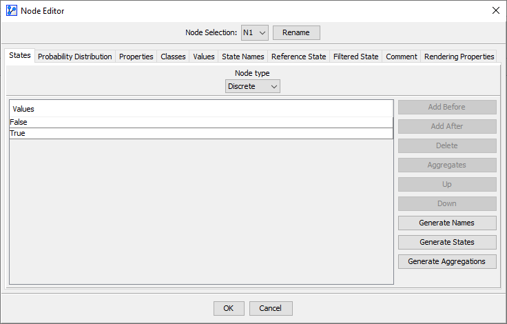
Discrete Nodes with Symbolic Values
- E.g., boolean , categorical {Low, Medium, High} or {red, green, blue}

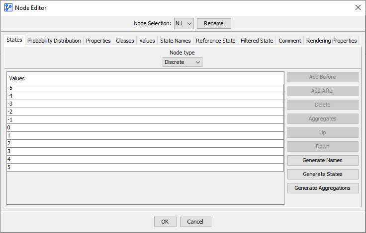
Discrete Nodes with Integer Values
- E.g., {-1, 0, 1, 2, 3, 4,…}

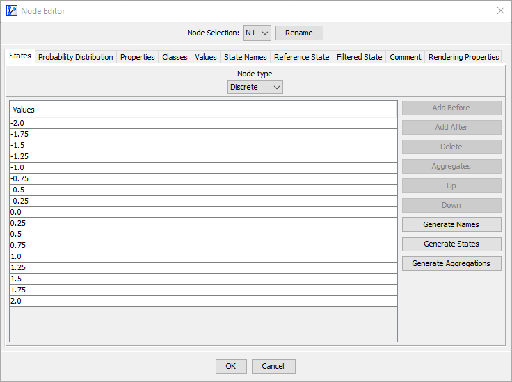
Discrete Nodes with Real Values
- E.g., {3.0, 3.25, 3.5,…}

Usage
Add Before/Add After
- The
Add BeforeandAdd Afterbuttons become available once you have selected any of the listed states.- Click on
Add Before, and BayesiaLab creates a new state before (i.e., above) the currently selected position on the list. - Clicking on
Add Afterproduces a new state after (i.e., below) the selected position.
- Click on
- The new states are automatically labeled L1, L2, L3, etc., regardless of the names of the existing states.
- By clicking into the list of states, you can overwrite existing or new node names.
Delete
- To delete a state, select it in the list and click the
Deletebutton. - Note that you can only delete one state at a time.
Up/Down
- Clicking the
UpandDownbuttons move the position of the state you have selected in the list. - This is useful for rearranging states with symbolic values so that they appear according to the natural order, e.g., Low, Medium, High.
Generate Names
- Clicking on the
Generate Namesbutton renames all the existing States with the default names L1, L2, L3, etc.
Generate States
- The
Generate Statefunction is very practical in the context of building new networks from scratch. - You can specify the number of new states to be generated, and then choose the naming convention or the numerical properties:
Automatic Namingproduces states with the automatically generated names, L0, L1, L2, etc.Numbered Names Prefixed bygenerates new states with names based on the string you specify followed by 0, 1, 2, etc.Integers Starting atcreates a series of states with integer values beginning with the specified value and increasing with the specified increments (must be integers of 1 or higher).Reals Starting atproduces a series of states beginning with the specified value and increasing with the specified real values (must be greater than 0)
Example & Workflow Illustration
-
The following animation shows Generate Names and Generate States in practice.
Aggregates & Generate Aggregations
Aggregation refers to the grouping of multiple states into a single state. This can be done as part of the Data Import process, or with this function at any time later.
This function is useful when dealing with a large number of discrete states in a node that would make it difficult to machine-learn relationships with that node.
The list of the aggregated states is used during Data Association for automatically associating these states with the defined state.
Manual Aggregation
- Click on
Generate Aggregations, which opens up the Aggregation Generator window. - From the list of states on the left, select the states you wish to aggregate using
Shift+ClickorCtrl+Click. - The newly-formed, aggregated state appears in the right list.
- By default, the original state names are concatenated using the ”+” symbol as a delimiter. An underscore ”_” is added as a prefix.
Example & Workflow Illustration
- In the following animation, we take the node , which includes all 50 U.S. states as Node States, and aggregate the states , , , , , and , into a new state, which we name .
Correlation-Aided Aggregation
In addition to the manual aggregation described above, BayesiaLab can support you in making the aggregation decisions. For this purpose, BayesiaLab can show how the original states of the to-be-aggregated node correlate with the states of other nodes on the Graph Panel.
Example & Workflow Illustration
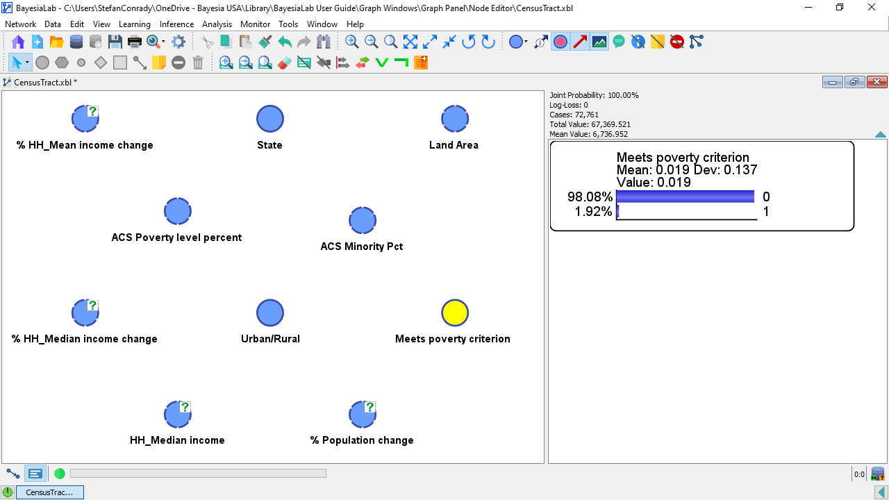
For illustration purposes, we utilize demographic data from 72,041 Census tracts across all 50 U.S. states. Let’s say we are developing public health policies for poor communities, and we know that roughly 2% of Americans live in Census tracts that meet the so-called poverty criterion. In this context, we’d like to reduce our original list of states and group them into three bins (or buckets) of states that have either no, some, or many poor communities. So, we need to aggregate 50 U.S. states into three aggregated sets of states.
Note that this is not the primary research objective. Rather, by creating this aggregation we want to facilitate a big-picture discussion about “rich states versus poor states” instead of looking at each state individually. Hence, we perform this aggregation before learning any network structure. So, the starting point is an unconnected network as shown in the screenshot below.

Example & Workflow Illustration
- In Modeling Mode
F4, open the Node Editor for the node . - Click the
Generate Aggregationbutton. - Click
Show Correlations. - Select
TargetandState. - Review
Correlations. - Manually select States to aggregate or click
Automatic Aggregation. - Click
Generate Aggregates. - Set the number of States and click
OKto confirm. - Review the new aggregated states and, if necessary, assign new names to replace the ones that were generated automatically.
- Click
OKto confirm. - Rearrange the order of States in the Node Editor, if appropriate.
- Click
OKto confirm.
Note that this type of aggregation cannot be reversed. All the original, underlying states are now merged into new states, and you won’t be able to undo this action.
