Evidence Instantiation

Context

• By definition, a Bayesian network represents a Joint Probability Distribution (JPD).
• Whenever you set any evidence on a network, the JPD becomes smaller, i.e., only a sub-space of the original JPD is now represented by the network given the evidence.
• For many research applications, you may only want to explore that very sub-space rather than the JPD as a whole.
• Evidence Instantiation provides a way to "extract" the sub-space of JPD as it is defined by the network and the evidence set.
• Evidence Instantiation creates a new network that represents only that sub-space of the original JPD.
• You may think that BayesiaLab achieves that by extracting a subset of the underlying dataset of the original network. However, that is not the case!
• Rather, the underlying dataset is irrelevant for Evidence Instantiation.
• Instead, Evidence Instantiation takes the original network structure and updates its Conditional Probability Tables so that it then represents the desired sub-space of the original JPD.

Usage & Example

• You can perform Evidence Instantiation based on any that has all Probability Tables and Conditional Probability Tables fully specified or estimated.
• Note that any type of evidence, including Soft Evidence and Hard Evidence, can be used in the context of Evidence Instantiation.
• To illustrate Evidence Instantiation, we use the familiar Perfume dataset, which we discuss in Chapter 8: Probabilistic Structural Equation Models of our e-book.

Perfume.xbl

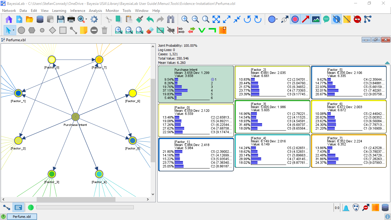
• In this example, we focus on the factor nodes, i.e., [Factor_0] through [Factor_7] .
  

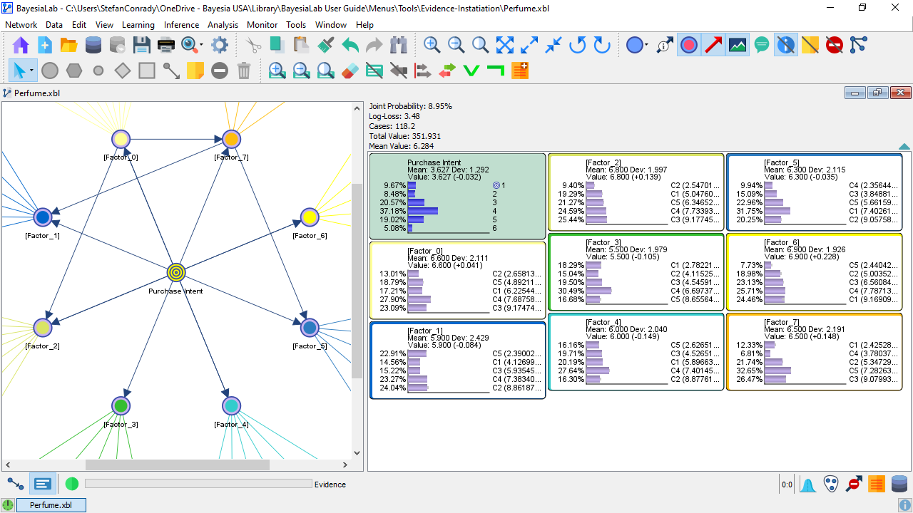
• Next, we set an arbitrary set of evidence on the factor nodes. For illustration purposes, we set Numerical Evidence using MinXEnt.
  

• Note the values reported in the Information Panel, right above the Monitor Panel:

  • No Evidence Set

  • Evidence Set

• The smaller value of the Joint Probability indicates that we are now looking at a sub-space of the original JPD.

• With this evidence set, we select Menu > Tools > Evidence Instantiation.

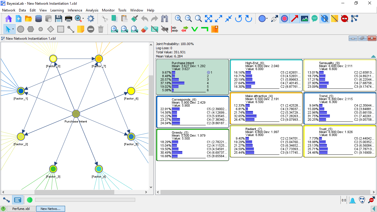
• This brings up a new Graph Window named New Network Instantiation 1.xbl.
  

• Please note the following points:

  • The factor nodes perfectly match the distributions set earlier as evidence.

  • However, these distributions are now marginal distributions, without any evidence set applied.

  • Also, the Information Panel now reports a Joint Probability of 100% again.

    • Evidence Set

    • Evidence Instatiation

  • So, the sub-space of the original JPD is now the entire JPD of the new network.

  • It is very important to know that there is no longer an associated database. The Graph Window of the original network featured the database icon to indicate that a dataset is associated with the network. Now, after the Evidence Instantiation, the icon is gone.

  • Also, the Information Panel showed the number of cases in the original dataset. With the Evidence Instantiation, the dataset was discarded, so there is no longer any reference to cases.

  • This also means that we would not be able to relearn the new network, as no data is available for that purpose.

  • However, we can perform inference on the newly instantiated network just like with any other network or the original network.