Dynamic Bayesian Networks
Graphical Representation
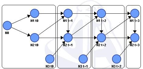
You can use a temporal dimension in the context of a static Bayesian network by “unrolling” the network to the desired number of time steps (i.e., by duplicating the network for each time step, as illustrated in the screenshot below for four time steps). However, this solution is only feasible for a limited number of time steps.
A Dynamic Bayesian Network provides a much more compact representation of such stochastic dynamic systems. The compactness is based on the following assumptions:
- The process is Markovian, i.e., the variables of time step t depend on a set of variables that belong to a limited set of former time steps (typically only on the previous time step t-1, i.e., a first-order Markovian assumption).
- The system is time-invariant, i.e., the probability tables do not evolve as a function of time. This last assumption is partially relaxed in BayesiaLab as the Time Variable makes it possible to modify the probability distributions based on the current time step with user-defined equations.
Given a first-order Markovian assumption, it is possible to represent such a system with only two time slices. The screenshot below shows the same network as the unrolled network presented above, but without any limitations on the number of time steps. The first slice describes the initial network at time step t0, and the second one describes the temporal transitions t+1.
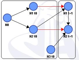
The t+1 slice is defined by Temporal Arcs (shown in red). A Temporal Arc indicates that the two connected nodes represent the same node at two consecutive time steps. As a result, the nodes in the t+1 slice are the destination nodes of the Temporal Arcs.
For a Markovian assumption of a higher order than one, the nodes of time slice t+1 are also linked to nodes belonging to time slices prior to time slice t0. However, Temporal Arcs can only be used to link nodes between time slices t0 and t+1.
The initial slice is particularly important because its synchronous arcs (connecting the nodes within the t0 slice, such as N0 -> N1 t0 and N0 -> N2 t0 in the example above) are removed after the first temporal inference. Then we have the common representation of a Dynamic Bayesian Network in which nodes of the t slice have no parents.
Inference
Inference in a Dynamic Bayesian Network is not as simple as with a static Bayesian network. BayesiaLab provides two types of inference:
-
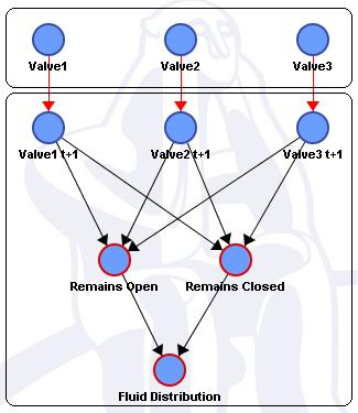
Inference based on a Junction Tree, which yields exact inference for static networks, but returns approximate results for dynamic networks. In special cases (e.g., the valve system shown below), the inference is exact because the valves are independent of each other. Similar to Bayesian Updating, obtaining exact results with dependent temporal nodes requires qualitatively indicating the dependencies without modifying the original conditional probability table. Simply add arcs between these dependent nodes, as illustrated below.
-
Inference based on Monte Carlo simulation (particle filtering), which yields approximate inference in the static and dynamic case. In both cases, the approximation is of the same order; that is, it is not related to node dependence and is only due to the randomness of the simulation.
Temporal Simulation
In Validation Mode, the toolbar has five new tools for temporal simulation:
-
 Resets the network. The synchronous arcs
and the probability tables of the t0 slice are reset. The network also resets
after entering new probability distributions for the temporal parent nodes and
when switching to Modeling Mode.
Resets the network. The synchronous arcs
and the probability tables of the t0 slice are reset. The network also resets
after entering new probability distributions for the temporal parent nodes and
when switching to Modeling Mode. -
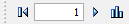
 The time meter indicates the current value
of the time step. This meter can also be used to enter the time steps to be reached,
i.e., the length of the simulation. If this value is lower than the current time
step, the network will be reset. Otherwise, the simulation is carried out from the
current time step to the set number. The simulation can be stopped by
clicking on the red light in the Status Bar. If a Temporal Evidence Scenario File
is associated with the network, right-clicking on the index field displays a list
of the evidence sets. Selecting a line performs the temporal simulation from the
current index to the specified index, taking into account the corresponding sets of
evidence:
The time meter indicates the current value
of the time step. This meter can also be used to enter the time steps to be reached,
i.e., the length of the simulation. If this value is lower than the current time
step, the network will be reset. Otherwise, the simulation is carried out from the
current time step to the set number. The simulation can be stopped by
clicking on the red light in the Status Bar. If a Temporal Evidence Scenario File
is associated with the network, right-clicking on the index field displays a list
of the evidence sets. Selecting a line performs the temporal simulation from the
current index to the specified index, taking into account the corresponding sets of
evidence: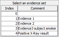
-

Simulates temporal step by temporal step.
-

Shows a graphical view of the probability evolution of the Temporally-Spied Nodes, as shown below.
If a Temporal Evidence Scenario File is associated with the network, the corresponding evidence for each time step will be taken into account. You can also add a set of evidence for the current time step by pressing  in the Monitor toolbar. Note that setting the probability distribution of a node depends on the chosen inference method: fixed distribution with exact inference, or computed likelihoods with approximate inference.
Sometimes a fixed probability distribution cannot be exactly achieved because the algorithm for computing the target distribution fails to converge. In this case, a warning is displayed, and a message is posted to the Console.
The Temporal Chart button displays the following window:

For each Spied State, the mean of the probability over the simulated period appears in the legend. If the network has utility nodes, the mean of the expected value of each utility node appears in the upper right corner, as well as the sum of these expected values.
Right-clicking on the graph brings up the Contextual Menu, which allows you to select the following:
- Show a relative view of the graph. The Y-axis shows the minimal and maximal values rather than the 0-to-100 scale, which is the default view.
- Print the graph.
- Copy the graph, which can then be pasted as an image or as a data array into external applications. Points can also be saved directly into a text file.