Network Performance Analysis Overall — Learning & Test Set
Context
- This Overall Performance Report evaluates a network with regard to a dataset that does have a Learning/Test Set split.
- If your dataset does not have a Learning/Test Set split, please see Report for Learning Set.
- Given that most performance measures here are the same as in the Report for Learning Set, we refer to that topic when appropriate rather than duplicating the content.
- In this topic, we focus on the additional features and objectives related to the Learning/Test Set split.
Notation
- denotes the Bayesian network to be evaluated.
- represents the entire Dataset associated with the Bayesian network . The Dataset is split into two partitions:
- represents the Learning Set of the Dataset from which network was learned.
- represents the Test Set (or holdout sample), i.e., the portion of the Dataset that will be used to evaluate network .
- represents an n-dimensional observation (Evidence), i.e., one row or record in the Learning Set , from which the Bayesian network was learned.
- represents an n-dimensional observation (Evidence), i.e., one row or record in the Test Set , which will be used to evaluate network .
- refers to the number of observations in the Learning Set .
- refers to the number of observations in the Test Set .
- refers to a Complete or fully connected network, in which all nodes have a direct link to all other nodes. Therefore, the complete network is an exact representation of the chain rule. As such, it does not utilize any conditional independence assumptions for representing the Joint Probability Distribution.
- represents a Unconnected network, in which there are no connections between nodes, which means that all nodes are marginally independent.
Example
To explain and illustrate the Overall Performance Report, we use a Bayesian network model that was generated with one of BayesiaLab’s Unsupervised Learning algorithms. This network is available for download here:
Overall Performance Report
The Report window consists of three tabs:
- Test Dataset
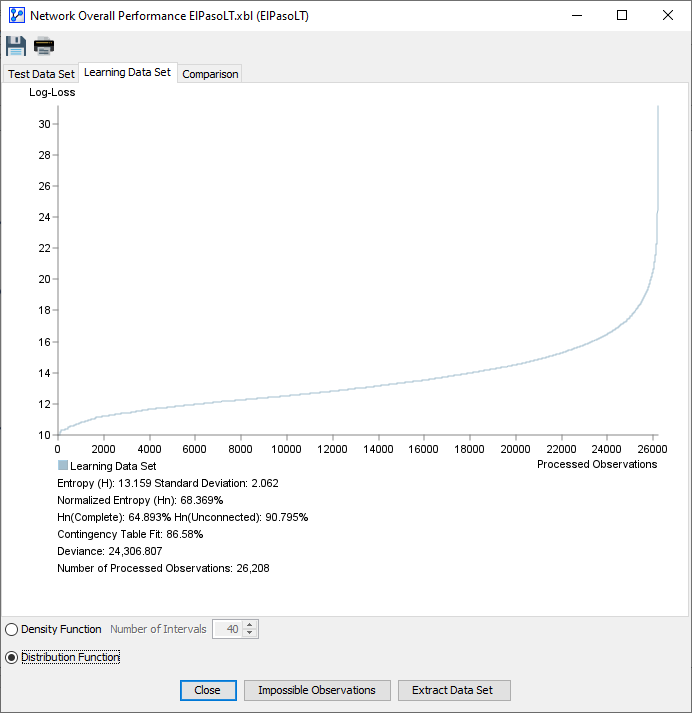
- Learning Dataset
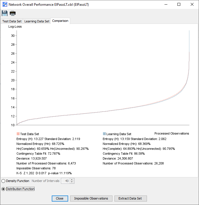
- Comparison
which feature two views each:
- Density Function
- The x-axis represents the Log-Loss values in increasing order.
- The y-axis shows the probability density for each Log-Loss value on the x-axis.
- Distribution Function
- The observations in the dataset are sorted in ascending order according to their Log-Loss values:
- The x-axis shows the observation number.
- The y-axis shows the Log-Loss value corresponding to each observation.
- The observations in the dataset are sorted in ascending order according to their Log-Loss values:
| Test Dataset Evaluation | Learning Dataset Evaluation | Comparison |
|---|---|---|
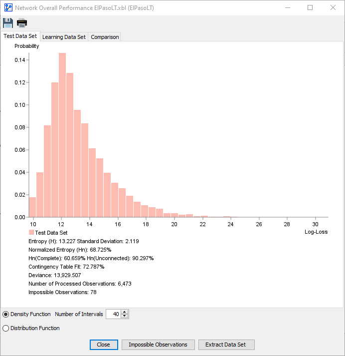 | 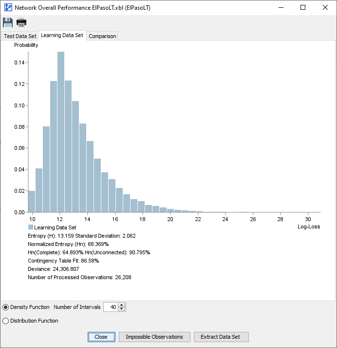 | 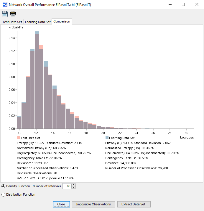 |
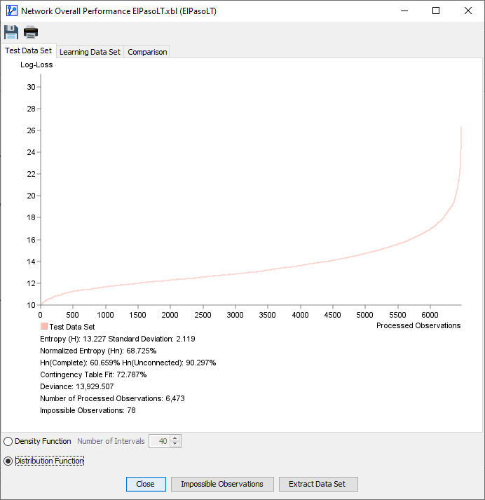 |  |  |
The radio buttons on the bottom-left of the window allow you to switch the view between the Density function (Histogram) and the Distribution function.
Either view provides a visualization of the Log-Loss values for all observations in the dataset given the to-be-evaluated Bayesian network . Thus, the plots provide you with a visual representation of how well the network fits the dataset .
Comparing Density & Distribution Functions
In the topic, Overall Performance Report for the Learning Set, the focus was primarily on how well the network fits dataset . All measures were about goodness-of-fit.
Our objective for this topic is broader. We are still looking for a good fit, but also want to understand how well the learned network model generalizes beyond the dataset from which it was learned.
In this context, the Comparison tab provides a key visual. You can see the histograms of the Log-Losses of the Learning Set and Test Set overlaid on top of each other.
Log-Loss Computation
The computation of Log-Loss values is at the very core of this Overall Performance Report. In the Report for Learning Set, the Log-Loss values were computed for the entire dataset .
Given the Learning/Test Set split, BayesiaLab now needs to compute all metrics separately for the Learning Set and the Test Set.
And, in addition to Log-Loss for the to-be-evaluated network , BayesiaLab also needs to compute the Log-Loss values for the complete network and Log-Loss for the unconnected network .
So, to produce the plots and all related metrics, BayesiaLab has to perform the following computations:
- , the Log-Loss value for each observation/evidence in the Learning Set based on the learned, to-be-evaluated Bayesian network .
- , the Log-Loss value for each observation/evidence in the Learning Set based on the complete network .
- , the Log-Loss value for each observation/evidence in the Learning Set based on the unconnected network .
- , the Log-Loss value for each observation/evidence in the Test Set based on the learned, to-be-evaluated Bayesian network .
- , the Log-Loss value for each observation/evidence in the Test Set based on the complete network .
- , the Log-Loss value for each observation/evidence in the Test Set based on the unconnected network .
The following Log-Loss Table is an extract of the first ten rows each from the Learning Set and the Test Set along with the computed Log-Loss values for each record:
Log-Loss Table
| Learning/Test | Month | Hour | Temperature | Shortwave Radiation (W/m²) | Wind Speed (m/s) | Energy Demand (MWh) | Log-Loss (Bayesian Network) | Log-Loss (Complete Network) | Log-Loss (Unconnected Network) | | --- | --- | --- | --- | --- | --- | --- | --- | --- | --- | --- | | | | | | | | | | | | | learning | 8 | 18 | 36.57 | 213.60 | 2.00 | 1574.00 | 13.43 | 14.68 | 21.96 | | learning | 8 | 19 | 36.04 | 105.91 | 1.90 | 1574.00 | 13.85 | 14.68 | 21.61 | | learning | 8 | 20 | 34.71 | 42.72 | 2.14 | 1485.00 | 12.13 | 11.87 | 19.41 | | learning | 8 | 21 | 33.94 | 0.00 | 2.75 | 1470.00 | 11.88 | 11.87 | 17.71 | | learning | 8 | 22 | 33.19 | 0.00 | 3.55 | 1378.00 | 11.89 | 11.09 | 17.72 | | learning | 8 | 23 | 32.38 | 0.00 | 4.21 | 1249.00 | 14.12 | 12.68 | 16.93 | | learning | 8 | 0 | 31.56 | 0.00 | 4.50 | 1110.00 | 13.05 | 12.36 | 16.94 | | learning | 8 | 2 | 29.66 | 0.00 | 4.90 | 975.00 | 11.22 | 11.68 | 14.66 | | learning | 8 | 3 | 29.02 | 0.00 | 4.60 | 944.00 | 10.91 | 11.36 | 14.66 | | learning | 8 | 5 | 27.16 | 0.00 | 3.11 | 927.00 | 11.29 | 10.98 | 14.65 | | ⁞ | ⁞ | ⁞ | ⁞ | ⁞ | ⁞ | ⁞ | ⁞ | ⁞ | ⁞ | | | | | | | | | Entropy | Entropy | Entropy | | | | | | | | | Mean | 13.16 | 12.49 | 17.48 | | | | | | | | | Std. Dev. | 2.06 | 1.34 | 2.15 | | | | | | | | | Minimum | 9.69 | 9.43 | 14.37 | | | | | | | | | Maximum | 30.88 | 14.68 | 30.89 | | | | | | | | | Normalized | 68.369% | 64.893% | 90.795% | | | | | | | | | | | | | | Learning/Test | Month | Hour | Temperature | Shortwave Radiation (W/m²) | Wind Speed (m/s) | Energy Demand (MWh) | Log-Loss (Bayesian Network) | Log-Loss (Complete Network) | Log-Loss (Unconnected Network) | | | | | | | | | | | | | test | 8 | 1 | 30.60 | 0.00 | 4.80 | 1031.00 | 13.41 | 14.68 | 16.90 | | test | 8 | 4 | 28.16 | 0.00 | 3.70 | 926.00 | 10.74 | 10.68 | 14.68 | | test | 8 | 15 | 33.20 | 318.62 | 2.56 | 1554.00 | 14.62 | 12.68 | 20.63 | | test | 8 | 18 | 32.71 | 192.24 | 2.13 | 1468.00 | 13.74 | 14.68 | 19.37 | | test | 8 | 0 | 27.09 | 0.00 | 4.75 | 1113.00 | 11.09 | 11.09 | 16.44 | | test | 8 | 1 | 25.87 | 0.00 | 7.53 | 1033.00 | 13.69 | 12.68 | 17.62 | | test | 8 | 4 | 23.27 | 0.00 | 8.90 | 928.00 | 15.82 | 14.68 | 15.77 | | test | 8 | 5 | 23.10 | 0.00 | 6.82 | 928.00 | 11.71 | 11.51 | 15.04 | | test | 8 | 14 | 28.61 | 353.33 | 3.19 | 1412.00 | 19.10 | ? | 19.35 | | test | 8 | 20 | 27.70 | 27.59 | 4.12 | 1459.00 | 12.39 | 12.09 | 19.00 | | ⁞ | ⁞ | ⁞ | ⁞ | ⁞ | ⁞ | ⁞ | ⁞ | ⁞ | ⁞ | | | | | | | | | Entropy | Entropy | Entropy | | | | | | | | | Mean | 13.23 | 12.41 | 17.41 | | | | | | | | | Std. Dev. | 2.12 | 1.31 | 2.14 | | | | | | | | | Minimum | 9.69 | 9.43 | 14.38 | | | | | | | | | Maximum | 26.07 | 14.68 | 30.85 | | | | | | | | | Normalized | 68.725% | 64.499% | 90.479% |
The complete Log-Loss Table serves as the basis for calculating the measures that are reported at the bottom of the report.
The measures reported at the bottom of the Test Set and Learning Set tab, are shown side by side on the Comparison tab:
For clarity, we match up the report’s labels to the notation introduced at the beginning of this topic and the corresponding definitions.
| Label in Report | Definition in Context of Test Set | Definition in Context of Learning Set |
|---|---|---|
| Entropy (H), i.e., mean of Log-Loss Values of all observations | ||
| Normalized Entropy (Hn) | ||
| Hn(Complete) | ||
| Hn(Unconnected) | ||
| Contingency Table Fit | ||
| Deviance | ||
| Number of Processed Observations |
Impossible Observations
Impossible Observations refer to observations/evidence in the Test Set , which are entirely incompatible with the network that was learned from the Learning Set .
Kolmogorov-Smirnov Test
The Kolmogorov-Smirnov Test (KS Test) is a common tool for comparing statistical distributions. Here, we use it to compare the distribution similarity between two samples, i.e., learning and test, so this test is only computed for the comparison panel.
More specifically, it compares the distributions of the Log-Losses. The values Z, D and the corresponding p-value are displayed.
Extract Data Set
The final element in the report window is the Extract Data Set button. This is a practical tool for identifying and examining outliers, e.g., those at the far end of the right tail of the histogram.
-
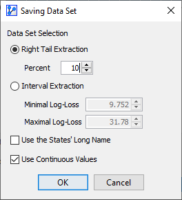
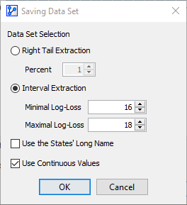
Clicking the Extract Data Set button brings up a new window that allows you to extract observations from the dataset according to the criteria you define:
-
Right Tail Extraction selects the specified percentage of observations, beginning with the highest Log-Loss value.
 Loading SVG...
 -
Interval Extraction allows you to specify a lower and upper boundary of Log-Loss values to be included.
 Loading SVG...
 -
Upon selecting either method and clicking OK, you are prompted to choose a file name and location.
-
BayesiaLab saves the observations that meet the criteria in CSV format.
-
Note that the Log-Loss values that are used for extraction are not included in the saved dataset.
