Prediction Analysis

Context

• The Prediction Analysis tool allows you to examine the predictive performance of a network model interactively.
• It generates a new causal network to represent the performance dynamics of the original model.
• This approach can help you interpret concepts such as precision, reliability, true/false positives, true/false negatives, etc.
• As a result, the usefulness of the model can be assessed and explained in detail.

Usage & Example

• Before you can initiate a Prediction Analysis, you need to have a network that was learned using Supervised Learning.
• Ideally, you would perform all other validation and performance testing steps, e.g., Structural Coefficient Analysis and Cross-Validation, before launching Prediction Analysis.
• For demonstration purposes, we show a Prediction Analysis based on a model for diagnosing coronary artery disease. We originally developed this model in a webinar on Diagnostic Decision Support.

• With this network active in the Graph Window, select Main Menu > Tools > Prediction Analysis.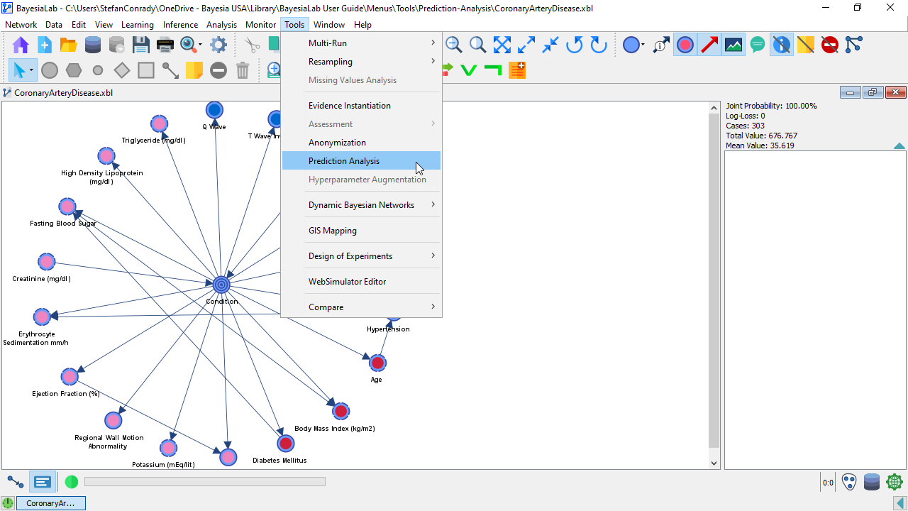

  

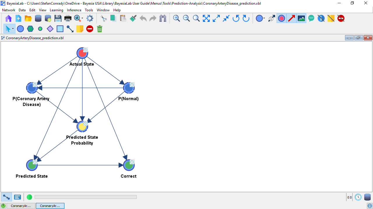
  Click to Zoom
  ×

  

• BayesiaLab generates a new model and opens a new Graph Window for it.

  

  Click to Zoom
  ×

  

• By default, BayesiaLab attaches the suffix “_prediction” to the original file name.

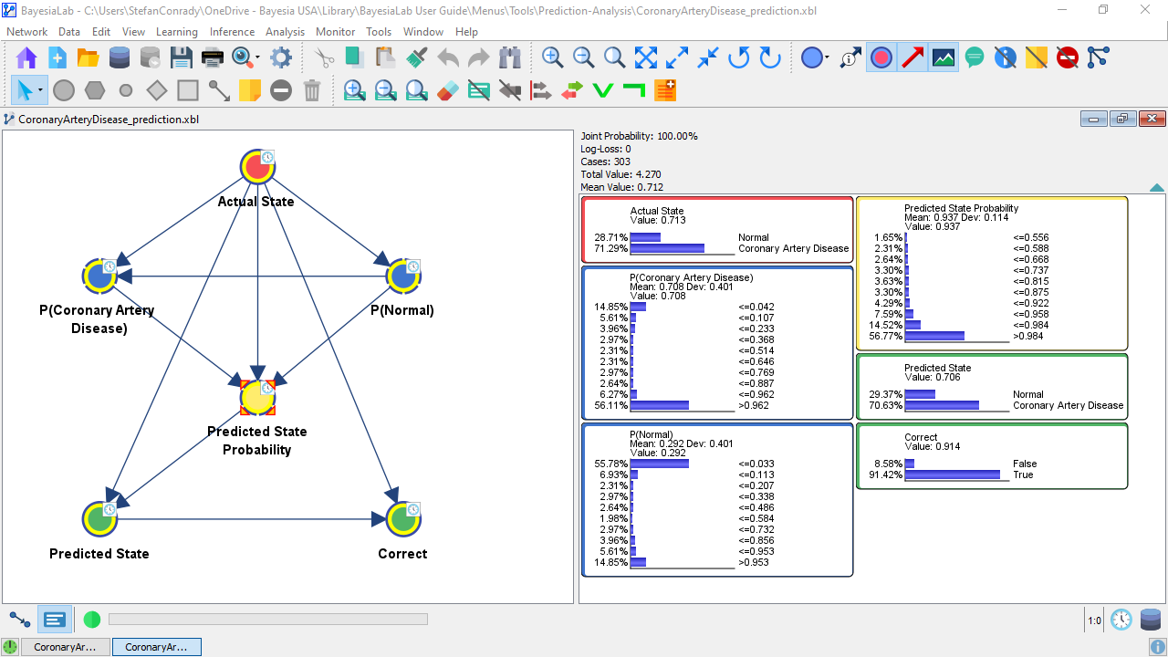
• Now, switch to the Validation Mode and bring up all nodes as Monitors in the Monitor Panel.

  

  Click to Zoom
  ×

  

• The node $\mathit{Actual\ State}$ represents the ground truth for the Target Node, i.e., the node $\mathit{Condition}$ in the network, which we are analyzing here.

• The nodes $P(\mathit{Coronary\ Artery\ Disease})$ and $P(\mathit{Normal})$ show the distributions of the probabilities predicted by the network for each state.

• The node $\mathit{Predicted\ State\ Probability}$ represents the probabilities associated with $\mathit{Predicted\ State}$. In other words, it shows the degree of confidence in the prediction. Given that this node represents the probability of the predicted state, the range of probabilities has to be $0.5 < \mathit{Predicted\ State\ Probability} < 1$. A probability below 0.5 would obviously imply that state would not be the predicted one.

• The node $\mathit{Predicted\ State}$ is the state the network predicted given the available observations.

• Finally, the binary node $\mathit{Correct}$ shows whether $\mathit{Predicted\ State}$ coincides with $\mathit{Actual\ State}$.

Interpretation

• The benefit of this model becomes clear once you translate common questions about the performance of a predictive model into queries of the corresponding prediction analysis model.

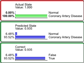
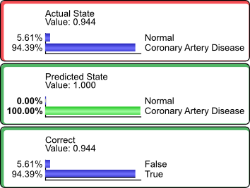
• For instance, we would be interested in how many of the patients who actually had Coronary Artery Disease were predicted as such. So, we set $P(\mathit{Actual\ State}=\mathit{Coronary\ Artery\ Disease})=100\%$.

  

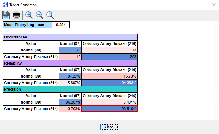
• We see that 93.52% of the cases of Coronary Artery Disease were predicted correctly.

• This value coincides with the Precision value (highlighted by the red border) reported in the Target Analysis Report.

  

• Conversely, we can set $P(\mathit{Predicted\ State}=\mathit{Coronary\ Artery\ Disease})=100\%$.

  

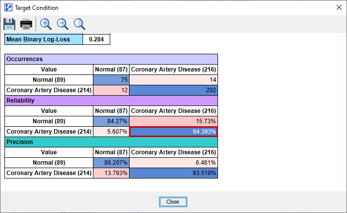
• This means that of those patients predicted to have Coronary Artery Disease, 94.39% did actually have the condition.

• This value coincides with the Reliability value (highlighted by the red border) reported in the Target Analysis Report.

  

• Similarly, any other cell in the Confusion Matrix above can be computed in the same way.

• Furthermore, we can pursue additional questions that cannot be easily obtained from any report.

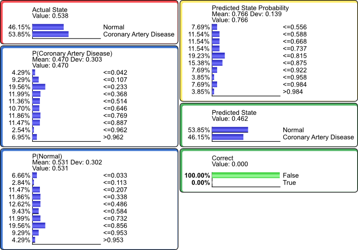
• For instance, we can examine the distributions that are associated with false predictions, by setting $P(\mathit{Correct}=\mathit{False})=100\%$.

  

• This would suggest that the distribution of false predictions is different from the marginal distribution of the actual state.

• In certain contexts, it can be valuable to understand the characteristics of false predictions for further refining the model.

Workflow Animation