Setting Evidence on Monitors

Context

We will now use this example to try out all types of evidence for performing inference.
One could certainly argue that not all types of evidence are plausible in the context of a Bayesian network that represents the stock market.
Within our large network of 459 nodes, we will only focus on a small subset of nodes, namely PG (Procter & Gamble), JNJ (Johnson & Johnson), and KMB (Kimberly-Clark). These nodes come from the “neighborhood” shown earlier.
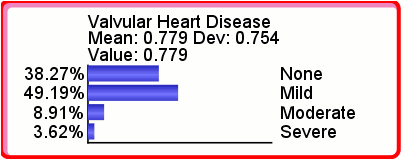
We start by highlighting PG, JNJ, and KMB to bring up their Monitors.
Prior to setting any evidence, we see their marginal distributions in the Monitors. We see that the expected value (mean value) of the returns is 0.

Hard Evidence

Probabilistic and Numerical Evidence

Given the discrete states of nodes, setting Hard Evidence is presumably intuitive to understand. However, the nature of many real-world observations calls for so-called Probabilistic Evidence or Numerical Evidence.

For instance, the observations we make in a domain can include uncertainty. Also, evidence scenarios can consist of values that do not coincide with the values of nodes’ states. So, as an alternative to Hard Evidence, we can use BayesiaLab to set such evidence.

Conflicting Evidence

In the examples shown so far, setting evidence typically reduced uncertainty with regard to the node of interest. Just by visually inspecting the distributions, we can tell that setting evidence generally produces “narrower” posterior probabilities.

However, this is not always the case. Occasionally, separate pieces of evidence can conflict with each other. We illustrate this by setting such evidence on JNJ and KMB. We start with the marginal distribution of all nodes.

After setting Numerical Evidence (using MinXEnt) with a Target Mean/Value of +1.5% on JNJ.

The posterior probabilities inferred as a result of the JNJ evidence indicate that the PG distribution is more positive than before. More importantly, the uncertainty regarding PG is lower. A stock market analyst would perhaps interpret the JNJ movement as a positive signal and hypothesize about a positive trend in the CPG industry. In an effort to confirm his hypothesis, he would probably look for additional signals that either confirm the trend and the related expectations regarding PG and similar companies.

In the KMB Monitor, the gray arrows and “(+0.004)” indicate that the first evidence increases the expectation that KMB will also increase in value. If we observed, however, that KMB decreased by 1.5% (once again using MinXEnt), this would go against our expectations.

The result is that we now have a more uniform probability distribution for PG—rather than a narrower distribution. This increases our uncertainty about the state of PG compared to the marginal distribution.

Even though it appears that we have “lost” information by setting these two pieces of evidence, we may have a knowledge gain after all: we can interpret the uncertainty regarding PG as a higher expectation of volatility.

Hard Evidence (Observation)

Hard Evidence refers to setting a particular state in a node to a 100% probability. This implies that all other states of the same node have to be at a 0% probability, as the probabilities of all states in a node must sum to 100%.

There are two ways to set Hard Evidence on Monitors.

Double-click on the probability bar of that state that you wish to set to 100%.
Right-click on the Monitor to bring up the Monitor

Upon setting Hard Evidence on a state, the corresponding bar appears in green and a 100% probability is shown

The observed node takes the green color of the observation.

Soft Evidence (Likelihood)

Setting Soft Evidence means modifying the probability distribution of a node.

The resulting relative likelihoods allow then computing, for each state, a factor used to update the probability distribution.

A node state with a zero likelihood value is an impossible state. If all the states have the same likelihood, the probability distribution remains unchanged.

There are two ways to set Soft Evidence:

Pressing the Shift key while clicking on the bar of a state.
Selecting Likelihood Evidence from the Contextual Menu of the Monitor.
- A green and red buttons are then added to the monitor. The likelihoods can be entered:
- by maintaining the left mouse button pressed while choosing the desired likelihood level, or
- directly by editing the likelihood value by double-clicking on the value.
Once all the likelihoods are entered, the light green button allows validating the data entry and the probability distribution is updated. The red button allows canceling the likelihood edition.

Setting likelihoods:

Result after validating with the light green button:

The observed node takes the light green color of the evidence.
With Likelihood Evidence, you can modify the Monitor's marginal distribution by applying a factor to the probability of each state.
Upon activating Likelihood Evidence, all factors are set to 1, which is represented by all bars set to 100%.
You can now adjust the bars with your mouse cursor and drag them to the desired levels. Alternatively, you can type in the percentage value.
Clicking the green button confirms your choice, and BayesiaLab displays a new, normalized distribution based on the original distribution, in which each state was multiplied by the specified factor.

Probability Setting

Setting the probabilities allows directly indicating the probability distribution of a node. Likelihoods are recomputed so that the final probability distribution of the node is the same as entered by the user.

The probability edition mode is available by two means: by pressing the Ctrl and Shift keys while clicking on a state bar or by using the contextual menu associated with the monitor. A light green, mauve and red buttons are then added to the monitor. The probabilities can be entered:

by maintaining the left mouse button pressed while choosing the desired probability level, or
directly by editing the probability value by double-clicking on the value.
A click on the name of the state (on the right) fix the current probability value (the probability bar is green).

Once all the probabilities are entered, the light green button allows setting the probabilities and the mauve button allows fixing the probabilities. The probability distribution is then updated. The red button allows canceling the probability edition.

So, there are two ways to use the probability capture:
Simply setting the probabilities: When the probabilities are validated with the light green button, the likelihoods associated with the states of the node are computed again in order to make the mar- ginal probability distribution correspond to the distribution entered by the user. It is, in fact, an indirect capture of the likelihoods. You must note that, at the next observation of another node, the probability distribution of this node will change because the likelihoods are not computed again.The result will be displayed with light green bars as the likelihoods:

The observed node takes the light green color of the evidence.

Fixing the probabilities: When the probabilities are validated with the mauve button, the likelihoods associated with the states of the node are computed again in order to make the marginal probability distribution correspond to the distribution entered by the user, as in the previous case. However, at each new observation on another node, a specific algorithm will try again to make the probability distribution of the node converge towards the distribution entered by the user. Fixing probabilities is also done in the evidence scenario files with the notation p{...} .You must note that fixing probabilities is only valid for the exact inference. If the approximate inference is used, fixing probabilities is considered like simply setting the probabilities: there is no more convergence algorithm. The result will be displayed with mauve bars:

The observed node takes the mauve color of the evidence.

To obtain the indicated distribution, a convergence algorithm is used. However, sometimes this algorithm cannot converge towards the target distribution. In this case, the probabilities fixing is not done and the node comes back to its initial state. In this case, a warning dialog box is displayed and an information message is also written in the console.

Setting a Target Mean/Value

When a node has values associated with states or is a continuous node or has numerical states, it is possible to choose a target mean/value for this node. An algorithm based on MinXEnt allows determining a probability distribution corresponding to this target mean/value, if this distribution exists. Of course, the indicated target value must be greater than or equal to the minimum value and less than or equal to the maximum value.

Once the target value entered, there are three options:

No Fixing: the distribution found must be observed as likelihoods.
Fix Mean: the indicated mean must be observed as fixed mean. When the mean is fixed, if an observation is done on another node, the convergence algorithm will automatically determine a new distribution in order to obtain the target mean, taking the other observations into account. If we store this evidence in the evidence scenario file, only the target mean will be stored. Fixing mean is also done in the evidence scenario files with the notation m{...}. You must note that fixing mean is only valid for the exact inference. If the approximate inference is used, fixing mean is considered like simply setting the likelihoods corresponding to the target mean: there is no more convergence algorithm.
Fix Probabilities: the distribution found must be set as fixed probability distribution. Fixing probabilities is also done in the evidence scenario files with the notation p{...}. You must note that fixing probabilities is only valid for the exact inference. If the approximate inference is used, fixing probabilities is considered like simply setting the likelihoods corresponding to the target mean: there is no more convergence algorithm.

Mean, Value, and Standard Deviations Hard Evidence