Example: Most Relevant Explanations for Failure Analysis

Example Background & Context

• To illustrate the Most Relevant Explanations function, we present a causal Bayesian network derived from a problem domain explained in Yuan, C. et al. (2011) , which had originally been proposed in Poole, D., & Provan, G. M. (1991).
• This domain was originally described as an electrical circuit consisting of an $Input$, an $Output$, and four switches, $A$, $B$, $C$, and $D$, which can fail.

Overhead Catenary System

• We took the liberty of embedding the problem Yuan described into a practical technical context, hoping to make it easier to understand.
• So, instead of a fictional and abstract circuit, we are considering an overhead catenary system that supplies power to electric locomotives along railroad tracks.

Conceptual Illustration

• Our system consists of the following elements, as illustrated in the above diagram.
  • A high-voltage wire, a so-called overhead catenary, serves as a power source for electric locomotives.
  • This high-voltage wire is suspended from a support structure that is attached to steel pylons alongside the railroad track.
• In addition to supporting the wire, this structure must also provide electrical insulation.
  • It does so through four insulators, labeled $A$, $B$, $C$, and $D$, so that there is no path along which electricity could flow into the steel pylon and ultimately into the ground.
  • As with all equipment that is exposed to the elements and subject to mechanical and electrical forces, these insulators can fail.
  • Long-term operational data has established specific failure probabilities for each of the insulators within a given time period:
    • $p(A=\mathit{defective})=1.6\%$
    • $p(B=\mathit{defective})=10\%$
    • $p(C=\mathit{defective})=15\%$
    • $p(D=\mathit{defective})=10\%$
  • In this context, “defective” means the degradation from a perfect insulator $(R = \infty)$ to an Ohmic resistor $(R \gg 0\,\Omega)$, not necessarily a short circuit $(R = 0\,\Omega)$.
• As a result, the failure of one or more insulators could create a stray current between the catenary wire ($\mathit{Input}$) and the steel pylon anchored in the ground ($\mathit{Output}$), thereby “leaking” electric energy.
• With that, the overall objective must be to prevent any stray currents. However, our specific objective in this example is to find the relevant causes if a stray current were to be observed.

Equivalent Circuit

• We can simplify the technical diagram from above into the following equivalent pseudo circuit, in which we represent the real-world insulators as idealized switches:

  • The equivalent of a functioning insulator is an open switch.
  • The equivalent of a defective insulator is a closed switch.

• Note that this circuit representation is identical to the one in Yuan’s paper.

• Looking at the arrangement of the insulators/switches, we can see that not all failures have the same effect:

  • A failure of $A$ would immediately create a connection between the $\mathit{Input}$ and the $\mathit{Output}$, leading to a power drain.
  • However, if any one of $B$, $C$, or $D$ failed by itself, it would not create an immediate problem.

• Beyond nodes that represent actual, technical components in our system, we introduce intermediate output nodes that inform us about the conditions on the output sides of the switches/insulators.

• Think of these intermediate output nodes as embedded sensors that indicate whether the corresponding switch can transmit power to the point where the sensors are attached:

• Here, the equivalent pseudo circuit is shown with the intermediate output nodes in place:

Explanatory Causal Bayesian Network

• Now we have all the elements we need to represent this domain in a causal Bayesian network:
  • $\mathit{Input}$ (i.e., the catenary) has the states $\mathit{Voltage}$ and $\mathit{No\ Voltage}$.
  • $\mathit{Output}$ (i.e., the pylon) has the states $\mathit{Current}$ and $\mathit{No\ Current}$.
  • The node names for the switches (i.e., the insulators) correspond to their designation in the diagram, i.e., $A$, $B$, $C$, and $D$. They all feature the states $OK$ and $\mathit{defective}$.
• The node names for the intermediate output nodes are $\mathit{Output}\ A$ through $\mathit{Output}\ D$. Each of them has the states $\mathit{Power}$ and $\mathit{No\ Power}$, indicating whether the respective switch can transmit power.
• Upon entering the failure probabilities, we have a fully specified causal Bayesian network, which you can download here:

Initial State of Bayesian Network

• Assuming that $\mathit{Input}=\mathit{Voltage}$, we can see how the Bayesian network computes the probability of $\mathit{Output}=\mathit{Current}$, i.e., the presence of a stray current.

System Failure Observed

• However, we are going to change the viewpoint. Instead of predicting the probability of system failure, we actually do observe a system failure, i.e., we measure a stray current that is flowing all the way to the $\mathit{Output}$.
• So, one or more of the components in this system must have failed.
• Unfortunately, we do not have access to the intermediate outputs, which would reveal what the problem is. Note that those nodes are marked as Not Observable.
• So, we must infer from the observed outcome and reason back to the potential causes.
• More specifically, we wish to know the most relevant causes, i.e., what would best explain the outcome we have observed.
• The following network illustrates the status of all nodes after setting $\mathit{Output}=\mathit{Current}$.

• Naively, we might expect that the node with the highest probability of being defective is the one that prompted the failure.
• However, the question is much more complex than that.

Most Relevant Explanations

• We need to employ the Most Relevant Explanations feature to identify the problems.

• Select Analysis > Report > Evidence > Most Relevant Explanations.

• This opens up an options window, in which we set the Search Space to the Ancestors of the Target Node $\mathit{Output}$.

  

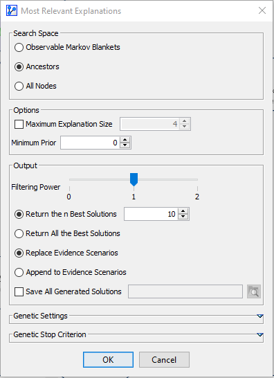
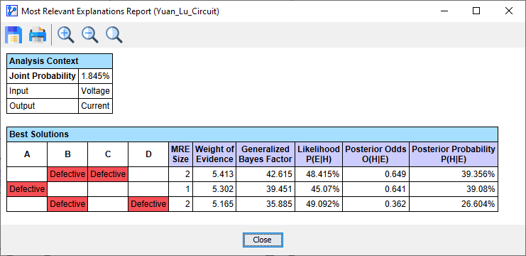
• Upon clicking OK, BayesiaLab starts the search and quickly brings up a report showing a list of solutions, i.e., explanations.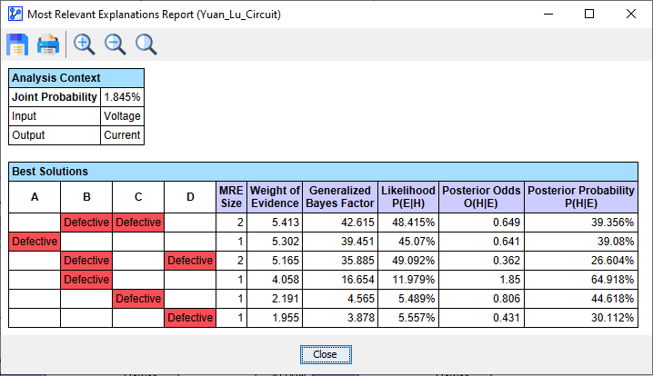

  

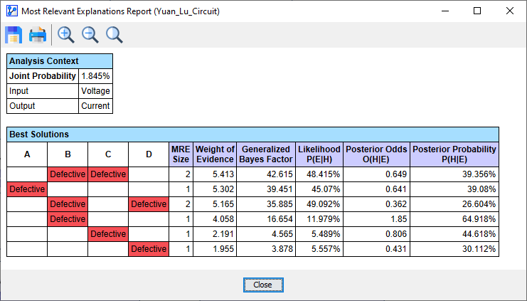
• In the list of Best Solutions, the top line shows the most relevant explanation $H^*$ for the observed evidence $E={\mathit{Input=Voltage}, \mathit{Output=Current}}$:

  • Both $\mathit{B}$ and $\mathit{C}$ are defective.

• Additionally, several measures corresponding to $H^*$ are reported in the columns to the right:

  • MRE Size refers to the number of individual pieces of evidence that are part of $H^*$, which is 2 for $B$ and $C$.
  • Generalized Bayes Factor (GBF): Given that our network is a causal model, we can use the likelihood ratio to interpret GBF. This means that the likelihood of $B=\mathit{defective}$ and $C=\mathit{defective}$ being the cause of $E$ is 42 times greater than the likelihood of $B=OK$ and $C=OK$ being the cause of $E$, i.e., 48.4% versus 1.1%.
  • Likelihood $P(E \mid H)$
  • Posterior Odds $O(H \mid E)$
  • Posterior Probability $P(H \mid E)$

Filtering Solutions

• In this example, the number of solutions is manageable. In more complex situations, however, the search algorithm could potentially find thousands of solutions.
• For constraining the size of the report, you can select the Filtering Power for producing the report.

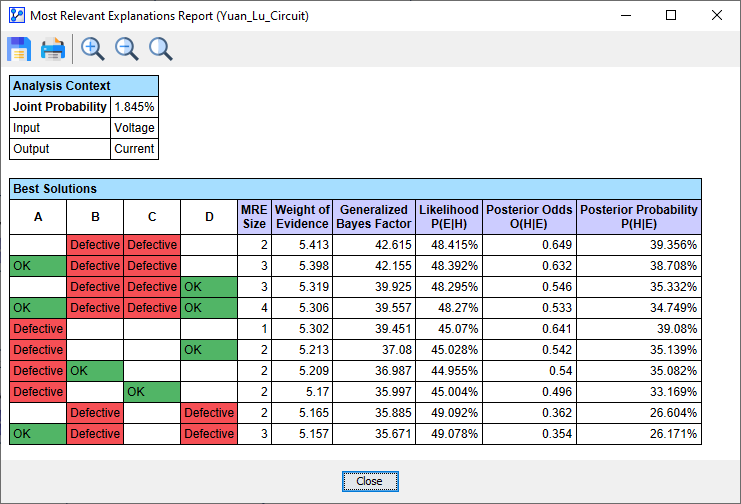
Filtering Power=0 (No Filtering)

Filtering Power=1 (Strongly Dominated Solutions are Filtered)

Filtering Power=2 (Strongly and Weakly Dominated Solutions are Filtered)

Workflow Animation