Example 1: Parameter Updating for One Node

• We start with a single node representing Sex, which has a uniform distribution, i.e., a 50/50 mix of Male and Female.

• For a compact presentation, we show the node Sex here in Monitor Style, which means that, in Validation Mode, the distribution of the states is directly shown on the node.

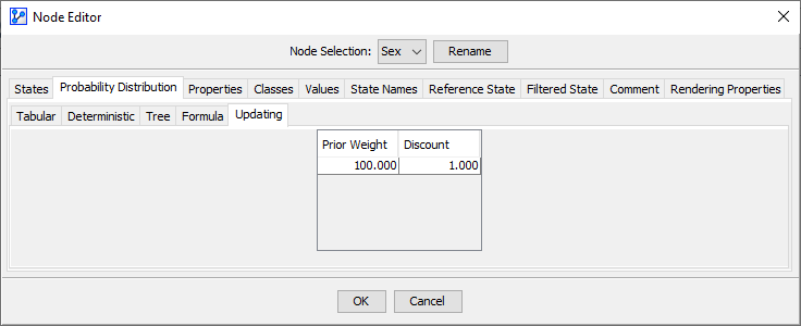
• Before starting Parameter Updating, we specify the Prior Weight and Discount via the Node Editor.

• Go to Node Context Menu > Edit > Probability Distribution > Updating.

• Here, we set the Prior Weight to 100. This means that we consider our prior equivalent to a population of 100 individuals, 50 male and 50 female.

• Furthermore, we leave Discount at its default value of 1. With this setting, we stipulate that no existing particles will be forgotten as additional new particles are added to the mix.

  

• Upon specifying these values, the node Sex is tagged with icons for Prior Weight and Discount .

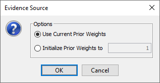
• You can start Parameter Updating in Validation Mode by selecting Menu > Inference > Parameter Updating.

• Then, a window prompts you to confirm the use of the currently specified Prior Weight or to select an alternative Prior Weight.

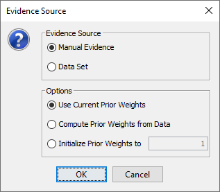
• If a dataset is associated with the given network, BayesiaLab will prompt you for additional settings:

• So, you can specify, for instance, that the Prior Weights be computed from the associated dataset.

• Additionally, you can choose the Evidence Source, which determines where to obtain the particles for Parameter Updating:

  • Manual Evidence means that new particles are coming from the evidence you set on the Monitors.
  • Dataset means that the observations stored in the associated dataset are retrieved to be used as particles.

• In this example, we continue with Manual Evidence.

• Upon clicking OK, a new control panel appears on the Toolbar.

  • takes the evidence entered via the Monitors and updates the probability tables accordingly.
  • removes all added particles and reverses any updates performed thus far.
  • Clicking activates the inclusion of Not-Observable Nodes from an associated dataset or an Evidence Scenario File. By default, observations of Not-Observable Nodes are excluded from updating probabilities in the context of Parameter Updating.
  • validates and saves all the updated probabilities and then closes Parameter Updating.
  • exits Parameter Updating without validating the updated probabilities. As a result, all updates are lost.
  • The counter shows how many particles have been added so far to update the probability tables.

Adding Particles

• We now take this network consisting of the single node Sex and perform Parameter Updating by adding particles one-by-one.
• All of the following screenshots focus on the relevant parts of the control panel in the Toolbar and the Monitor Panel.

Particle #1

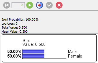
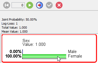
• For the first particle, we set the evidence Sex=Female.
• The Information Panel shows that the Joint Probability of _Sex=Female* is 50%, which is what we expect given the Probability Table we specified.
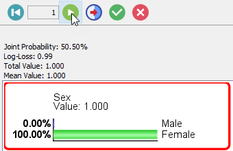
• Upon clicking , this new particle is mixed with the 100 virtual particles from the prior, and we now have a population of 51 females and 50 males.
• As a result, the probability table of the node Sex is updated using Maximum Likelihood Estimation based on this new population.
• The new probability of the state Female is now 50.5%. While we don't see the probability table of the node Sex, the Information Panel reports a Joint Probability of .
• Note that after adding the particle, the evidence remains set on Female.

Particle #2

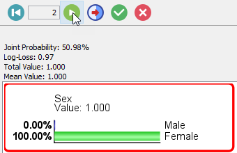
• Upon clicking , this evidence, i.e., Sex=Female, is added as a new particle and mixed with the 101 virtual particles, and we now have a population of 52 females and 50 males.
• The new probability of the state Female is now 50.98% and the Information Panel reports a Joint Probability of .
• Note that after adding the particle, the evidence remains set on Female.

Particle #3

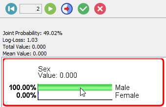
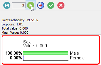
• Now for the third particle, we set the evidence Sex=Male.

• Upon clicking , this evidence, i.e., Sex=Male, is added as a new particle and mixed with the 102 virtual particles, and we now have a population of 52 females and 51 males.

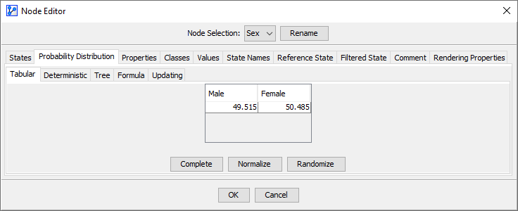
• The new probability of the state Male is now 49.51% and the Information Panel reports a Joint Probability of .

• Clicking and then confirming the prompt validates all three updates.

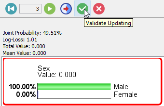
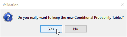
• Upon validation, we can immediately see the new marginal probability distribution for Sex, both on the node (in Monitor Style) and in the corresponding Monitor in the Monitor Panel.

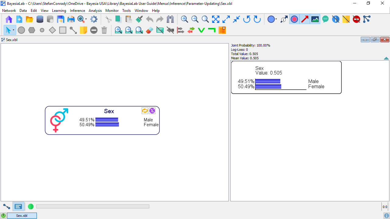
• Furthermore, we can go into the Node Editor to see its updated status.

• The Node Editor shows that the Prior Weight is now equal to 103:

  • 100 from the virtual particles defined via the original Prior Weight.

  • 3 from the particles we created by manually setting evidence.

    

  • Of course, we can also see the new marginal probability distribution in the Tabular tab.

Discounting

• With Discount set to 1, we did not apply any discounting to earlier particles as newer particles came in.
• Had we used a Discount of 0.75 instead, the Prior Weights and probabilities would have evolved as shown in the following table: