Degree of Freedom Reduction Efficiency

Context

• The Degree of Freedom Reduction Efficiency is available to be plotted within the Curve window as part of the Structural Coefficient Analysis.
• The Degree of Freedom Reduction Efficiency is denoted ηdf  and measures how the network complexity affects the quality of representing the associated dataset.
• As such, the Degree of Freedom Reduction Efficiency is closely related to the Contingency Table Fit (CTF), which quantifies the representation quality of the associated dataset.
• Formally, the Degree of Freedom Reduction Efficiency is defined as , where
  • is the degree of freedom of the fully connected network C.
  • is the degree of freedom of the current network B that corresponds to the current Structural Coefficient.
  • is the Contingency Table Fit of the current network B that corresponds to the current Structural Coefficient.

Usage

• To illustrate the Degree of Freedom Reduction Efficiency measure, we use a sample network that represents the joint probability distribution of physicochemical properties in a specific type of white wine. The dataset, on which this model is based, is available from the UCI Machine Learning Repository (opens in a new tab).​

WhiteWine.xbl

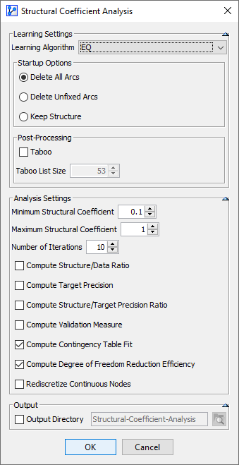
• On this network, we perform a Structural Coefficient Analysis: Main Menu > Tools > Multi-Run > Structural Coefficient Analysis.
• We follow the overall workflow introduced in Structural Coefficient Analysis.
• Given that the Degree of Freedom Reduction Efficiency is particularly relevant in the context of Unsupervised Learning, we use EQ as the Learning Algorithm.
• In addition to computing the Degree of Freedom Reduction Efficiency, we also check Contingency Table Fit.
• We set the Structural Coefficient to a range of 0.1 to 1.
  
• Upon clicking the Curve button at the bottom of the report, we obtain the following plot.
• In the screenshot below, the Contingency Table Fit is shown in red, and the Degree of Freedom Reduction Efficiency is displayed in green.
  
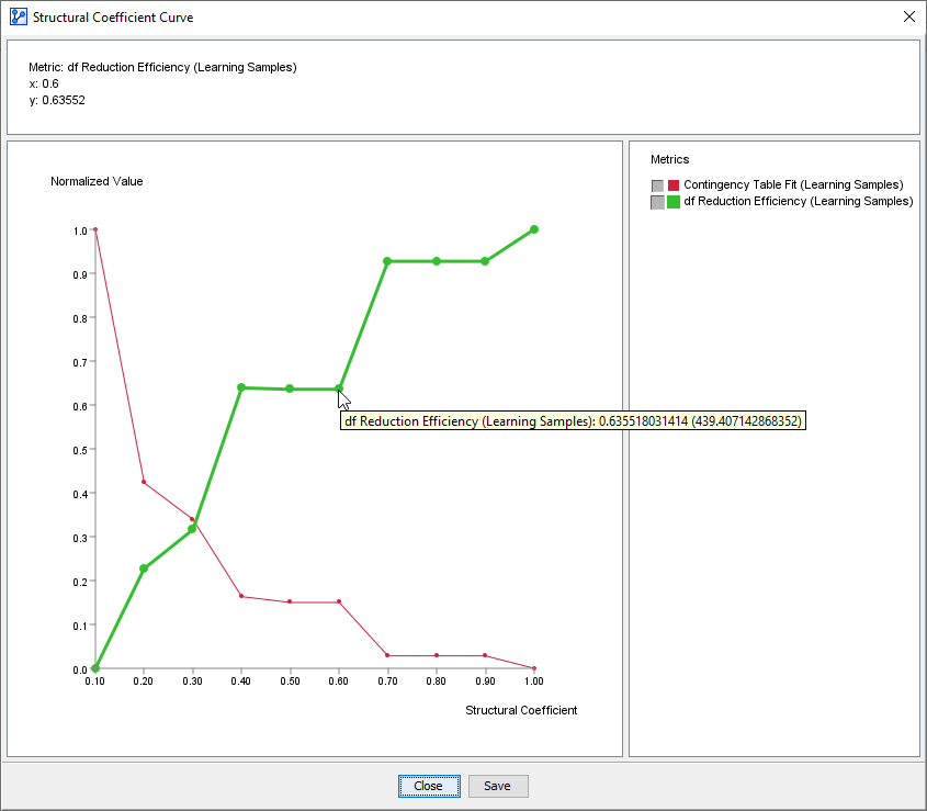
• The x-axis represents the Structural Coefficient values.
• The y-axis shows the Contingency Table Fit and the Degree of Freedom Reduction Efficiency computed for each network learned with the corresponding value of the Structural Coefficient.
• Note that the y-values are normalized to a 0-to-1 range for each curve separately.
• You can hover with your pointer over the points on the plot, and a tooltip will show the normalized value plus the unnormalized value in parentheses.

Interpretation

• At first glance, the Degree of Freedom Reduction Efficiency curve appears to mirror the Contingency Table Fit curve.
• To put these values in an even broader context, we set the Structural Coefficient to an extreme range of 0.01 to 150, which are the minimum and maximum values BayesiaLab allows for the respective fields, and run the Structural Coefficient Analysis again:
  
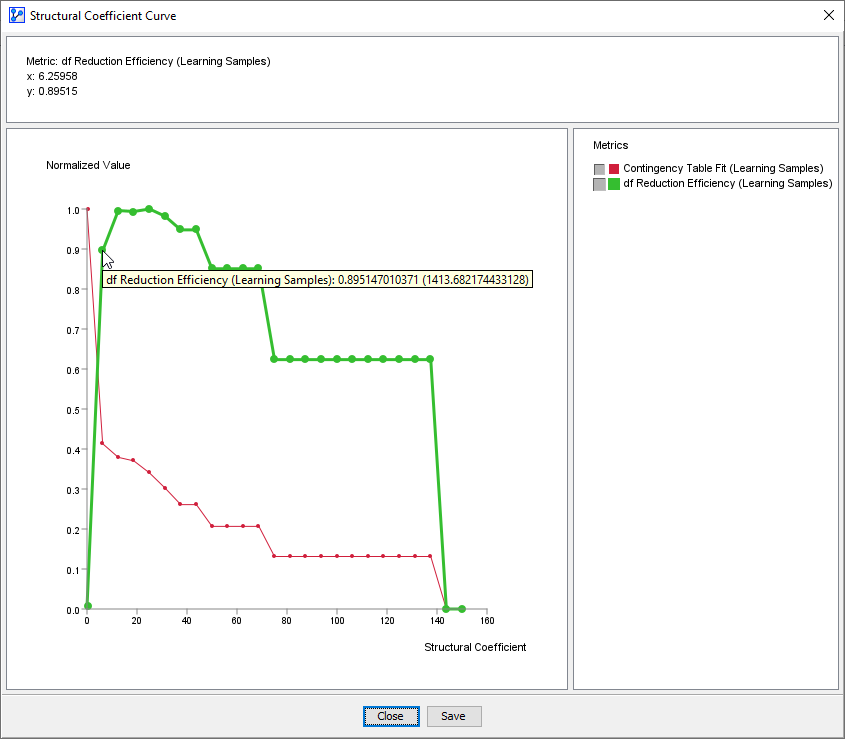
• This "big picture" provides a sense of how the Degree of Freedom Reduction Efficiency curve and the Contingency Table Fit curve are related.
• Whereas the Contingency Table Fit only informs about the quality of the representation,
• The rightmost point for the Contingency Table Fit at SC=150 implies that there is no network structure at all and hence the quality of representation is at its minimum.
• Given the absence of a network structure, there can't be any reduction in the Degree of Freedom. So, SC=150 marks a minimum for the Degree of Freedom Reduction Efficiency, too.
• As discussed under Contingency Table Fit, moving along the x-axis to the left shows a steadily increasing quality of representation, as the complexity of the network grows.
• The increase in network structure not only brings about a higher quality of data representation but also results in a more compact representation of the data.
• Thus, the Degrees of Freedom are reduced, and efficiency is gained.
• Both Degree of Freedom Reduction Efficiency and Contingency Table Fit move almost in parallel across a large range of Structural Coefficient values.
• As the Structural Coefficient approaches 0, both curves change their respective directions: Contingency Table Fit shoots to 1, and Degree of Freedom Reduction Efficiency drops to 0.
• This is the point where additional complexity can indeed produce an arbitrarily high quality of representation.
• However, instead of discovering regularities that would allow a compact representation, a disproportionate amount of complexity is required for a "pixel-perfect" representation of the data.
• As a result, the initial efficiency gain from creating a network structure now collapses to zero.
• So, at SC=0, we find a seemingly perfect representation of the dataset, which, however, is burdened by a tremendous overhead in complexity.
• This means that a network at SC=0 uses enormous complexity to model noise in the data and obscures any regularities in the dataset.
• While an overview of this 0-to-150 range provides context, in practice we focus on a much narrower range, typically from just above 0 up to the low single digits.
  
• Now understanding what each curve represents, we can use the zoomed-in view on the 0.1-to-1 range to help find and appropriate values for the Structural Coefficient.
• The objective is to find a Structural Coefficient value that yields a good-quality representation of the data while maintaining a high degree of abstraction, i.e., a high Degree of Freedom Reduction Efficiency by virtue of having a model.
• Given these considerations, the range could be appropriate for choosing a Structural Coefficient value.
• While it is certainly helpful for selecting a Structural Coefficient value, you should consider this plot only in the context of all the other measures produces by the Structural Coefficient Analysis.