Sensitivity Analysis — Joint Probability
Background & Motivation
- When we hear analysts discussing elections, we often hear about “core voters” and “swing voters” and their respective roles in election results.
- By using these terms, such analysts implicitly perform a Joint Probability Analysis on the voter base.
- Let’s assume that in a two-party race, Party A vs. Party B, the candidate of Party A wins the election with 51% of the votes. Therefore, the marginal probability that a voter votes for Party A must be 51%.
- Theoretically, it is possible that 51% of all voters are absolutely determined to vote for Party A, while 49% are dead set on Party B. With such immutable convictions, an election campaign would be unnecessary.
- However, the very existence of the terms “core voter” and “swing voter” implies that the probability of voting for Party A is not the same across all voters. Core voters will vote for Party A with a high degree of certainty, while swing voters might be swayed either way.
- For an election campaign, it is critical to understand how many voters remain on the proverbial fence, as they can perhaps be moved to their side. A similar challenge exists in marketing, i.e., to know how much conquest potential exists among current consumers of a competitive brand.
- In such a context, the objective of BayesiaLab’s Joint Probability Analysis is to decompose the overall 51% vote for Party A into its “sources,” i.e., core voters and swing voters.
- We will return to the election example in the Usage section, but first we need to explain the fundamentals with a simple example.
Bayesian Network Context
- The probabilities associated with Root Nodes in a Bayesian network are easy to understand. Root Nodes only have outgoing arcs, but no incoming arc.
- As a result, a Root Node only needs a Probability Table that contains the marginal probabilities of its states.
- However, the probabilities of states of nodes that have incoming arcs, i.e., all Child Nodes, are not defined directly. Rather, Child Nodes are only defined conditional on their Parent Nodes.
- Thus, inference is required to obtain the marginal probabilities of the states of Child Nodes.
Introductory Example: Eye Color & Hair Color
-
In the following example, we have a simple network consisting of the Parent Node, , and the Child Node, , which are connected by an arc.
Loading SVG... -
Given that has no ancestors, it is a Root Node, and given that has no descendants, it is a so-called Leaf Node.
-
We can see that the probabilities of the states of are specified conditional on the states of . Thus, we require a Conditional Probability Table, not just a Probability Table.
-
Of course, if we have the Probability Table of and the Conditional Probability Table of , we can infer the marginal probabilities of the states of , too, even though those probabilities are not directly recorded anywhere in the Bayesian network.
-
Therefore, we can consider the inferred marginal distribution of as a “summary” calculated on the fly by BayesiaLab to show in the corresponding Monitor:
Loading SVG... -
More specifically, the marginal probability of is the result of a calculation that is equivalent to the following equation. To simplify the notation, we use the shorthand for , etc.:
-
As a result, we automatically obtain a decomposition of the marginal probability of . We learn what “makes up” by looking at the individual terms in the above equation. We find, for instance, that brown-eyed folks are the biggest “source” of black hair.
-
For more complex networks, of course, this approach is not feasible. Think of a network that also includes ethnicity, gender, age, geography, culture, fashion trends, beauty ideals, etc.
-
Now we need BayesiaLab’s Joint Probability Analysis to decompose which combinations of attributes “produce” blonds, for instance. While the “blond hair and blue eyes” stereotype may still hold, there may also be unlikely sources of blonds.
Joint Probability Analysis
- Using BayesiaLab’s Joint Probability Analysis, we can decompose the marginal distribution of any node or nodes, however complex the network, and visualize their composition. In this context, we will refer to such nodes as Target Nodes.
- The nodes on which the Target Nodes depend are called Parameter Nodes. In our example, is a Target Node and is a Parameter Node.
- While it is certainly excessive to perform a Joint Probability Analysis on our simple example, it will help us understand the mechanics of this analysis.
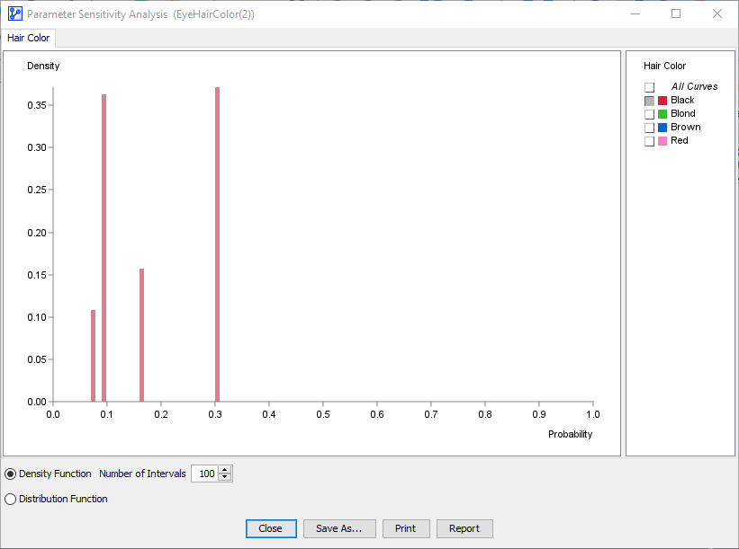
- The Joint Probability Analysis generates a histogram that allows us to decompose the marginal probabilities on the Target Node , and shows them relative to the Parameter Node .
- The following screenshot shows the histogram for the state :
- The illustration below shows how the histogram links the probabilities in the Conditional Probability Table of the Target Node, , to the Probability Table of the Parameter Node, :
- The x-position of the bars shows the probability of the state given the states of the Parameter Node .
- The y-values of the bars show the probability of each state of the Parameter Node occurring.
- We need to think of each state of the node , i.e., Brown, Hazel, Blue, and Green, as a scenario. So far, each scenario consists just of a single state.
- Later, scenarios will consist of combinations of states of multiple Parameter Nodes. Thus, we will need to refer to the Joint Probability of scenarios involving multiple Parameter Nodes, rather than the probability of one state of a single Parameter Node.
- So, what do we gain with this type of visualization? In this simple example, probably not much at all.
- However, if a Target Node does not depend on a single Parameter Node, but on dozens of Parameter Nodes in a Bayesian network, this histogram can help us visually decompose the marginal distribution of the Target Node. In a more complex network, the Joint Probability Analysis may have to evaluate millions of scenarios in a Bayesian network upon which Target Nodes depend.
- In our example, the Target Node only depends on the four states of the Parameter Node . Thus, each histogram bar represents one state (or scenario).
- More specifically, BayesiaLab has to compute the posterior probabilities of the Target Nodes for each scenario and the Joint Probability of each scenario.
- Alternatively, BayesiaLab can sample from all possible scenarios and infer the posterior probabilities of the Target Nodes on the sampled subset.
- Then, the histogram aggregates the Target Nodes’ posterior probabilities into bins along the x-axis.
- By virtue of sampling from the joint distribution of scenarios, the y-values of the histogram bars represent the Joint Probability of the scenarios corresponding to the probability bin on the x-axis.
- In other words, we can see what Joint Probabilities of scenarios correspond to which posterior probabilities of the Target Node states.
- The example in the Usage section will provide more intuition why this can be helpful for understanding Target Nodes.
Practical Example: 2012 Presidential Election
- We now return to the election campaign example and employ a model based on the 2016 General Social Survey in this context.
- The General Social Survey contains questions about a wide range of social and political issues. Furthermore, the survey includes a question about who survey respondents voted for in the 2012 presidential election, i.e., Mitt Romney or Barack Obama.
- Based on this data, we can machine-learn a simple Bayesian network that predicts the presidential vote based on a subset of social and political beliefs.
- The following screenshot shows this model in Validation Mode
F5. The Monitor displays the marginal distribution of the Target Node PRES12.
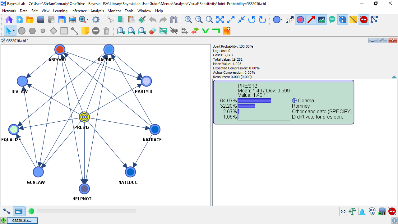
Note that this network is not meant to serve as an example of an optimal predictive model. The purpose of this network is to illustrate Joint Probability Analysis rather than to show how to fine-tune its performance.
-
For your reference, this predictive Bayesian network model is available for download here:
GSS2016.xbl -
However, our objective is not the prediction itself. Rather, we want to understand the probability of voting one way or another for the entire spectrum of thousands of possible belief scenarios.
-
This way, we hope to understand where the votes came from, i.e., the core or swing voters.
Usage
-
To start the Joint Probability Analysis, go to
Main Menu > Analysis > Visual > Sensitivity > Joint Probability. -
In the options window, you need to specify several items:
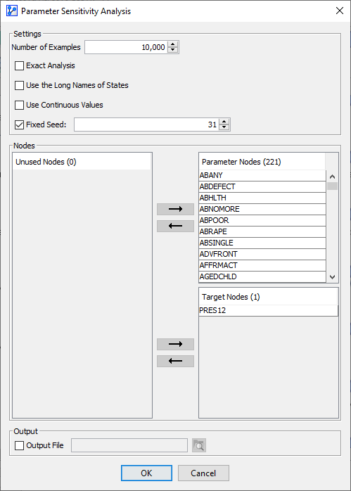
- Number of Samples: This is the number of samples to be drawn to represent the Joint Probability Distribution of the Parameter Nodes. We specify 10,000 samples.
- Exact Analysis: By checking this box, you can force BayesiaLab to exhaustively evaluate all possible combinations of states of the Parameter Nodes. As you check this box, the Number of Samples field displays the exact number of cases to be generated.
- Use the Long Names of States: This option allows you to display the Long Names of states in the report. However, you also have the option of switching to Long Names in the report window later.
- Fixed Seed: Setting a Fixed Seed allows you to perform the same random draws each time you run the analysis.
- In the three panels in the center of the window, you need to specify the role of all nodes for this analysis:
- Parameter Nodes: The Parameter Nodes serve as the basis for the scenarios to be evaluated. By default, Root Nodes would be assigned to the list of Parameter Nodes.
- Apart from the Target Node, we select all nodes in the network as Parameter Nodes.
- Altogether, the combinations of states of these 9 Parameter Nodes can constitute 30,240 possible scenarios. If we checked Exact Analysis, all of them would be evaluated.
- Target Nodes: The Target Nodes are the nodes of interest, i.e., we want to learn how their marginal probability distributions can be decomposed.
- By default, Leaf Nodes are added to the list of Target Nodes.
- Furthermore, if a Target Node is formally defined, it will be assigned to the group of Target Nodes as well.
- In our example, the Target Node in the Bayesian network model is also the only Target Node here for the purpose of the analysis.
- Unused Nodes: Any node on the list of Unused Nodes is available to be assigned to the Parameter Nodes or the Target Nodes. Nodes remaining on the list of Unused Nodes will be omitted from the analysis.
- Parameter Nodes: The Parameter Nodes serve as the basis for the scenarios to be evaluated. By default, Root Nodes would be assigned to the list of Parameter Nodes.
- Under Output, you can specify an output file in CSV format, which records the inferred probabilities of the Target Nodes for each scenario.
- If the analysis is performed using sampling, the sampled scenarios implicitly represent the Joint Probability Distribution.
- If Exact Analysis is checked, the output file also includes a field explicitly stating the Joint Probability of each scenario. This is necessary as scenarios generated for Exact Analysis are an exhaustive list of all combinations of states of all Parameter Nodes. Thus, the list would not represent the Joint Probability Distribution of the Parameter Nodes, which the sampling approach automatically generates.
- The following screenshot shows all available options for the analysis:
-
Click
OK, and BayesiaLab generates the scenarios and infers the posterior probabilities for the Target Nodes. -
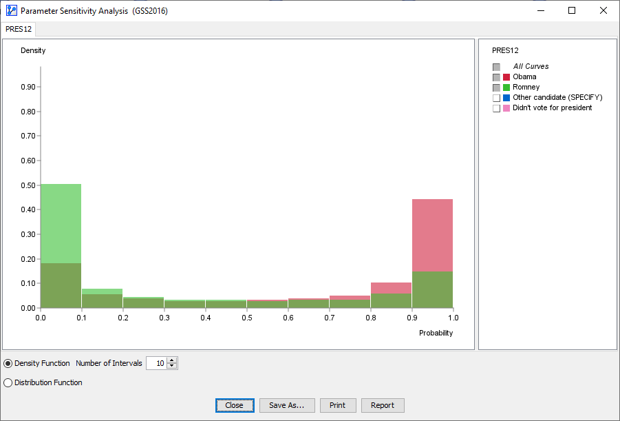
A report window opens and features the histogram we discussed earlier.
-
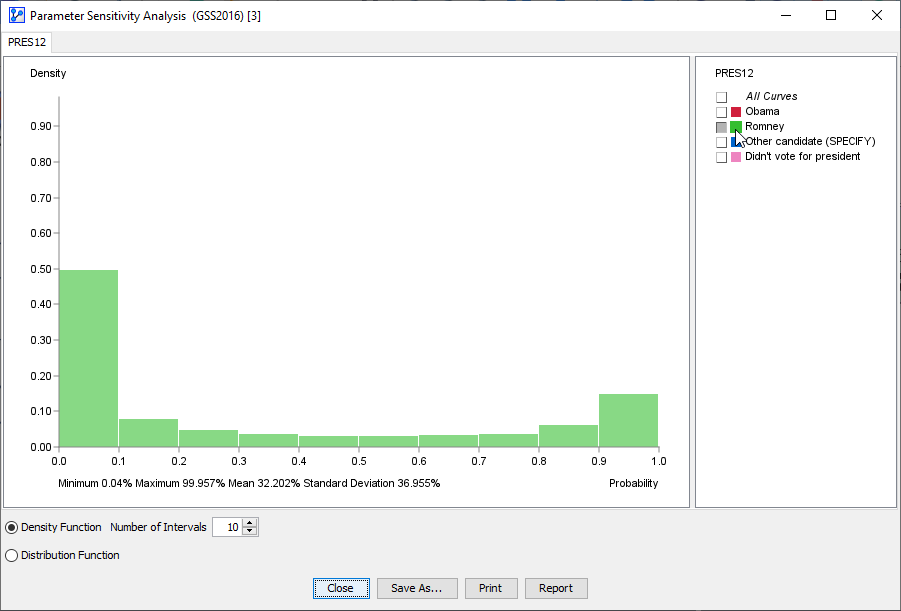
In this histogram, we only focus on the probabilities associated with votes for Obama and Romney.
-
Furthermore, we reduce the default number of intervals from 100 to 10.
-
The following animation displays the probabilities of the Romney vote.
-
As the cursor moves across the histogram bars, the Tooltip shows two percentages in parentheses, e.g.,

- The first value represents the probability interval of the Target Node.
- The second value shows the Joint Probability of the scenarios that constitute the bar.
- For example,
 means that in 14.85% of all scenarios, the probability of voting for Romney fell into the 90 to 100% range.
 - On the other end of the spectrum,
 means that in over half of the scenarios, the Romney vote was in the 0 to 10% probability range.
-
We now have the desired decomposition of the marginal probability of the Romney vote.
-
Also, by hovering over the Romney field in the legend, BayesiaLab reports the overall statistics of the Romney vote probabilities:
-
Minimum: 0.04%
-
Maximum: 99.957%
-
Mean: 32.202%
-
Standard Deviation: 36.955%
-
While the mean value is indeed 32.2%, it would correctly represent the probability of voting for Romney for only about 3.5% of voters.
-
As we can see in the histogram, our model suggests a high degree of polarization.
-
So, if this analysis were based on pre-election surveys, the opportunity for swaying the swing voters toward Romney would be limited.
-
The middle ground of probabilities around the 50% mark appears quite thin.
-
