Multiple Clustering

Context

Multiple Clustering performs data clustering on subsets of variables in a Bayesian network.

The subsets are defined by classes named [Factor_i].

The nodes in each class [Factor_i] are used to induce a new node — a latent variable — which summarizes the underlying manifest nodes.

You can manually define classes to be used for Multiple Clustering, but they can also be created automatically using Variable Clustering.

A Bayesian network is created for each of these classes. This network contains the variables that belong to the class and the synthetic variable Cluster named [Factor_i]. This variable is added to the corresponding class [Factor_i] and set as Not Observable. If the initial network contains fixed arcs, they are added to each new Bayesian network if they are included in it, i.e., the extremities of each arc are contained in the network. At the end of the last data clustering, a final Bayesian network is created. It contains all the Clusters and comes with an internal database where all the values of these latent variables have been inferred with respect to their corresponding network. It is also possible to add the initial variables (the manifest variables) to that final Bayesian network.

The following dialog box allows entering the parameters for Multiple Clustering. It automatically reuses most of the parameters used for data clustering.

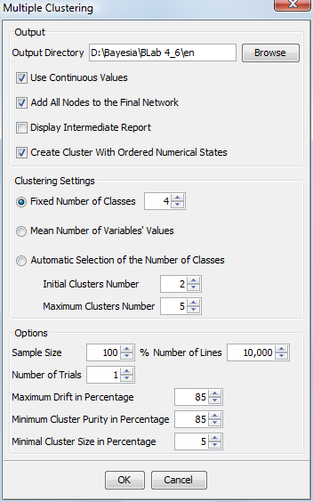
In the Output area, the wizard allows selecting the directory where the various generated networks will be saved (a network by class [Factor_i] and the final network with all the latent variables). The intermediate and final databases are saved with the generated networks. The continuous values can be saved with the databases. This wizard also allows you to add or exclude the nodes of the initial network in the final one. It is also possible to display or hide the intermediate report generated for each intermediate network. However, the intermediate reports are always saved in the target directory.

It is possible to create, for each network, a cluster node with ordered numerical states. These values are the mean of the score of each connected node for each state of the cluster node. If two of these values are strictly identical, an epsilon is added to one of them to obtain two different values.

As in Data Clustering, the number of values of the latent variables can be a priori fixed or found by a random walk. It can also be defined as being equal to the average number of values of the variables belonging to [Factor_i]. The remainder is strictly identical to Data Clustering.

At the end of each clustering, an algorithm automatically determines if one of the [Factor_i] node’s states is a Filtered State. If so, this state is marked as filtered.

At the end of each clustering, an automatic analysis of the obtained Bayesian network is carried out and a target analysis report is generated. This report is identical to the one generated by Data Clustering. It can be displayed if the relevant option is selected. However, it is always saved in the target directory.

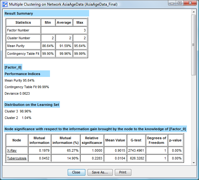
At the end of the last clustering, a synthesis report is generated. At the beginning of the report, a summary indicates the number of factors found, and the minimum, average, and maximum number of clusters, mean purity, and contingency table fit.

This report describes, for each latent variable, the mean purity, Contingency Table Fit, and Deviance. Those indices are described in the Correlation with Target Node’s report. This new measure can be used to qualify the clustering result, to measure how well the Joint Probability Distribution is represented through each [Factor_i] variable.

It also describes the distribution of its values on the learning set, and the list of the nodes sorted according to the quantity of information brought to its knowledge (cf. Target analysis report). The final network is automatically opened and the final database is associated with it. If the initial database contains a test set, it is also transferred and the missing value imputation is performed on the new [Factor_i] variables. Finally, the final database is saved in the target directory.