Contingency Table Fit

Context

• The Contingency Table Fit is available to be plotted within the Curve window as part of the Structural Coefficient Analysis.
• Contingency Table Fit (CTF) measures the quality of the representation of the Joint Probability Distribution by a Bayesian network B in comparison to a complete (i.e., fully-connected) network C and a fully-unconnected network U.
• BayesiaLab's CTF is formally defined as:

where

• is the entropy of the data with the unconnected network U.

• is the entropy of the data with the evaluated network B.

• is the entropy of the data with the complete (i.e., fully-connected) network C. In the complete network, all nodes are directly connected to all other nodes. Therefore, the complete network C is an exact representation of the chain rule. As such, it does not utilize any conditional independence assumptions for representing the Joint Probability Distribution.

• As such, the CTF is an excellent measure to examine the relationship between complexity and data representation.

• As with all measures provided by the Structural Coefficient Analysis, the Contingency Table Fit supports you in choosing an appropriate value for the Structural Coefficient.

Usage

• To illustrate the  Degree of Freedom Reduction Efficiency measure, we use a sample network that represents the joint probability distribution of physicochemical properties in a specific type of white wine. The dataset, on which this model is based, is available from the UCI Machine Learning Repository (opens in a new tab).​

WhiteWine.xbl

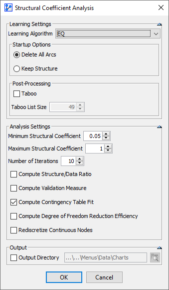
• On this network, we perform a Structural Coefficient Analysis: Main Menu > Tools > Multi-Run > Structural Coefficient Analysis.
• We follow the overall workflow introduced in Structural Coefficient Analysis.
• Given that the Contingency Table Fit is particularly relevant in the context of Unsupervised Learning, we use EQ as the Learning Algorithm.
• We set the Structural Coefficient to a range of 0.05 to 1.
  
• Upon clicking the Curve button at the bottom of the report, we obtain the following plot.
• In the screenshot below, we have 10 x-y pairs (corresponding to 16 iterations) shown on the plot:
  
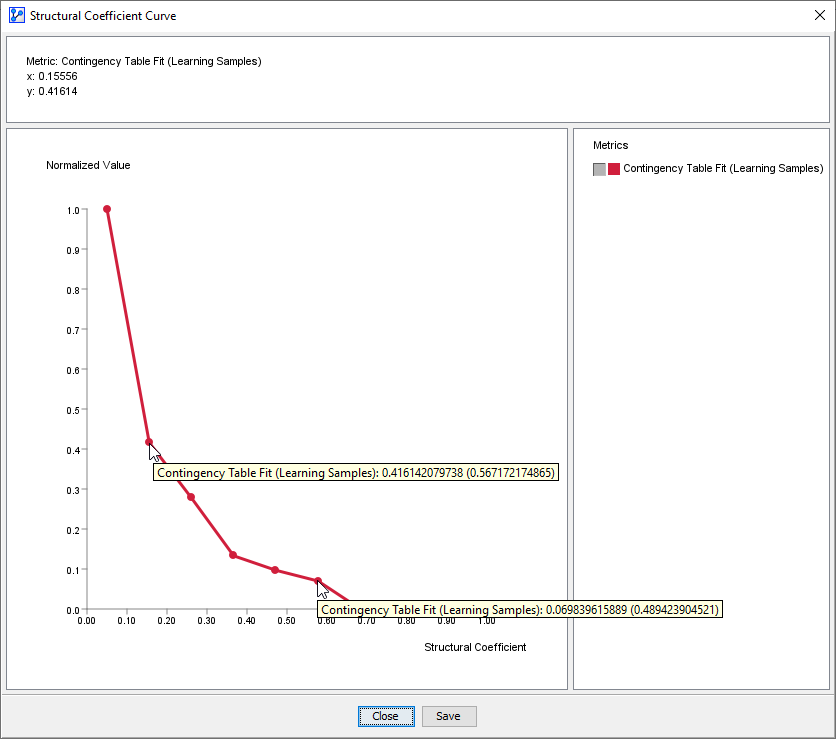
• The x-axis represents the Structural Coefficient values.
• The y-axis shows the Contingency Table Fit computed for each network learned with the corresponding value of the Structural Coefficient.
• Note that the y-values are normalized to a 0 to 1 range, i.e., the smallest computed Contingency Table Fit is displayed as 0 and the largest value as 1.
• You can hover with your pointer over the points on the plot, and a tooltip will show the normalized CTF value plus the unnormalized CTF value in parentheses.

Interpretation

• For , the CTF increases fairly steadily as the Structural Coefficient decreases.
• The two arbitrarily selected points on the curve show CTF values of 57% and 49% respectively.
• Here, we can see that adding model complexity (by lowering the Structural Coefficient) does steadily improve the data representation.
• These values need to be understood in context:
  • CB is equal to 100% if the Joint Probability Distribution is represented without any approximation, i.e., the entropy of the evaluated network B is the same as the one obtained with the complete network C.
  • CB is equal to 0% if the Joint Probability Distribution is represented by considering that all the variables are independent, i.e., the entropy of the evaluated network B is the same as the one obtained with the unconnected network U.
  • CB can also be negative if the parameters of network B do not correspond to the dataset.
• So, in the context of this theoretical 0–100% range, the different between 57% and 49% appears fairly substantial.
• To put these values in an even broader context, we set the Structural Coefficient to an extreme range of 0.01 to 150, which are the minimum and maximum values BayesiaLab allows for the respective fields, and run the Structural Coefficient Analysis again:
  
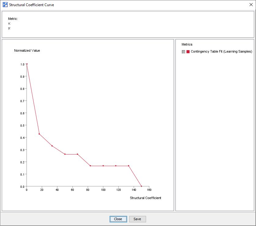
• Now, the normalized scale of the plot and the absolute CTF values coincide:
  • SC=0 → CTF=100%
  • SC=150 → CTF=0%
• This means that our analysis of the 0.1-to-1 range earlier "zoomed in" on a tiny section of this "big picture."
• This "big picture" can give you a sense of "how much traction" a model can gain with regard to a dataset.
• As in the zoomed-in plot, we can see that adding model complexity (by lowering the Structural Coefficient) does indeed steadily improve the data representation.
• In other words, the model's structure can capture regularities in the data and represent them.
• So, for choosing an appropriate value of the Structural Coefficient, we are looking for the maximum y-value on a steady slope on the curve while avoiding the explosive growth towards 0, which is indicative of overfitting.
• This approach is similar to interpreting the Structure/Data Ratio, where we are looking for the inflection point in the curve but have to stay clear of overfitting.

Overfitting

• For comparison, a model that is ill-suited to given the dataset would show little improvement in terms of data representation until it reaches the stage of overfitting, at which point the model is fitting noise as opposed to regularities in the data.
• The following plot illustrates this situation. Here, we perform a Structural Coefficient Analysis on pure noise, i.e., nodes with random distributions:
  
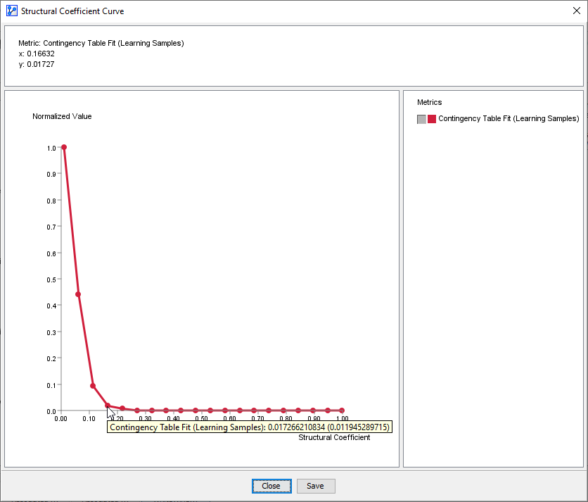
• So, reducing the Structural Coefficient does produce a meaningful represtantion of the dataset.
• Only as the Structural Coefficient is approaching 0, the model appears to generate some degree of data representation.
• Given that we know that the underlying dataset is pure noise, any apparent data representation is a prototypical example of overfitting.
• It illustrates the old adage, "if you torture the data long enough, it will ultimately confess."