Profile Analysis

Context

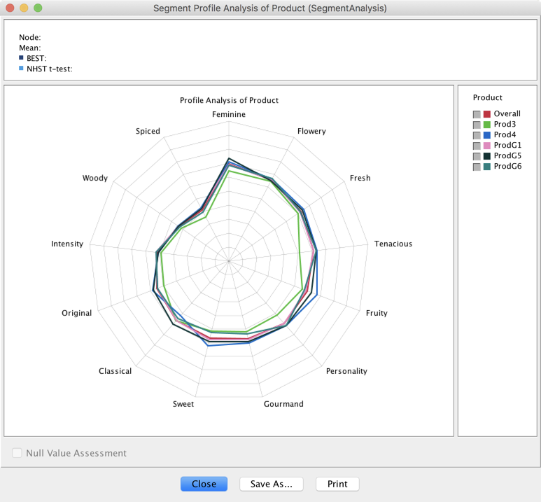
The Profile Analysis feature allows you to compare the mean values of observable variables for the segments defined by the Breakout variable.

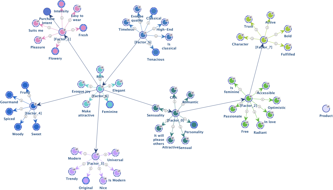
Let’s take the Perfume example for which we have defined five segments with the Breakout Variable $\mathit{Product}$ , namely $\mathit{Prod3}$ , $\mathit{Prod4}$ , $\mathit{ProdG1}$ , $\mathit{ProdG5}$ , and $\mathit{ProdG6}$ .

When two segments are selected, this option allows estimating whether the mean values of these segments are significantly different.
Two tests are proposed for answering this question:
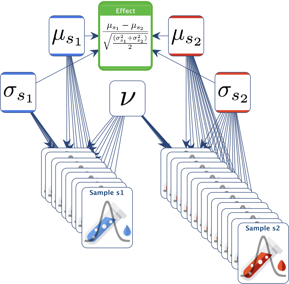
- A frequentist one: NHST t-test (Null Hypothesis Significance Testing) with Welch’s two-sample, two-tailed t-test.
- A Bayesian one: BEST, described in the paper by John K. Kruschke, “Bayesian Estimation Supersedes the t-test”, Journal of Experimental Psychology: General, 2013.
Below is the Bayesian network used in the BEST approach. We assume that the samples follow a Student’s t-distribution. The two segments have their own $\mu$ and $\sigma$ , but they share the same $\nu$ .
The default Confidence Level has been set to 95%. This is the same for both tests.
As for the Bayesian test, the Region of Practical Equivalence (ROPE) on the effect size around the null value has been set by default to [-0.1, 0.1].
The null value is rejected if the 95% Highest Density Interval (HDI) falls completely outside the ROPE.
You can use the Preferences to modify:
- the confidence level (for both the t-test and BEST),
- the Markov Chain Monte Carlo parameters used for inference in the Bayesian network described above,
- the ROPE size that defines an interval centered at 0, i.e., 0.2 defines the interval [-0.1, 0.1].

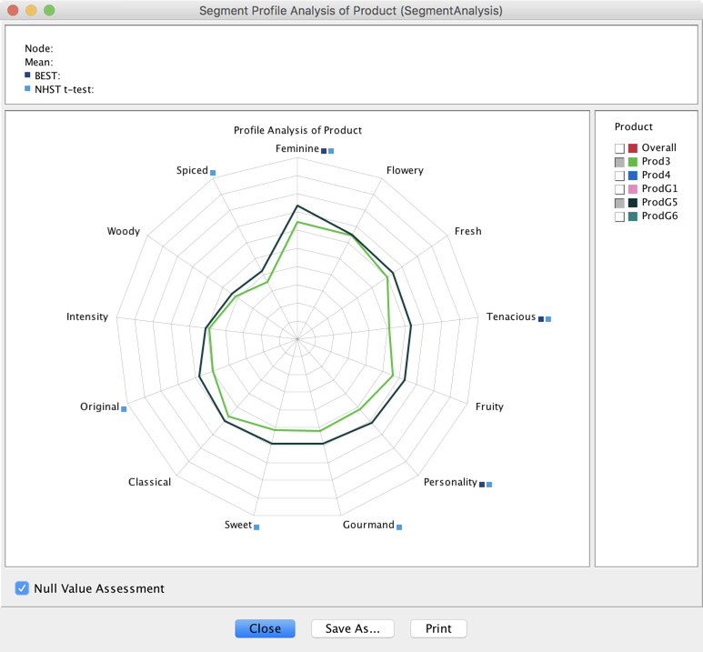
We first select $\mathit{Prod3}$ and $\mathit{ProdG5}$ . Upon checking Null Value Assessment, the computation of both tests is triggered.
If the mean values are estimated as significantly different, a square is added next to the label:
- for the t-test
- for BEST