Network Performance Analysis Overall — Learning Set

Context

This Overall Performance Report evaluates a network with regard to a dataset that does not have a Learning/Test Set split.
If your dataset does have Learning/Test Set split, please see Report for Learning and Test Set.

Notation

$B$ denotes the Bayesian network to be evaluated.
$D_L$ represents the Dataset from which network $B$ was learned.
$E_L$ represents $E$ evidence. Evidence refers to an n-dimensional observation, i.e., one row or record in the dataset $D_L$ , from which the Bayesian network $B$ was learned.
$N_L$ refers to the number of observations $E_L$ in the dataset $D_L$ .
$C$ refers to a Complete or fully connected network, in which all nodes have a direct link to all other nodes. Therefore, the complete network $C$ is an exact representation of the chain rule. As such, it does not utilize any conditional independence assumptions for representing the Joint Probability Distribution.
$U$ represents an Unconnected network, in which there are no connections between nodes, which means that all nodes are marginally independent.

Example

To explain and illustrate the Overall Performance Report, we use a Bayesian network model that was generated with one of BayesiaLab's Unsupervised Learning algorithms. This network is available for download here:

ElPaso.xbl

Overall Performance Report

Density & Distribution Function

The top part of the Report features a plot area, which offers two views:

Density Function
- The x-axis represents the Log-Loss values in increasing order.
- The y-axis shows the probability density for each Log-Loss value on the x-axis.
Distribution Function
- The observations $E$ $E$ in the dataset $D$ $D$ are sorted in ascending order according to their Log-Loss values:
  - The x-axis shows the observation number.
  - The y-axis shows the Log-Loss value corresponding to each observation.

Click on the thumbnail images to enlarge the screenshots of each view:

Density Function (Histogram)	Distribution Function

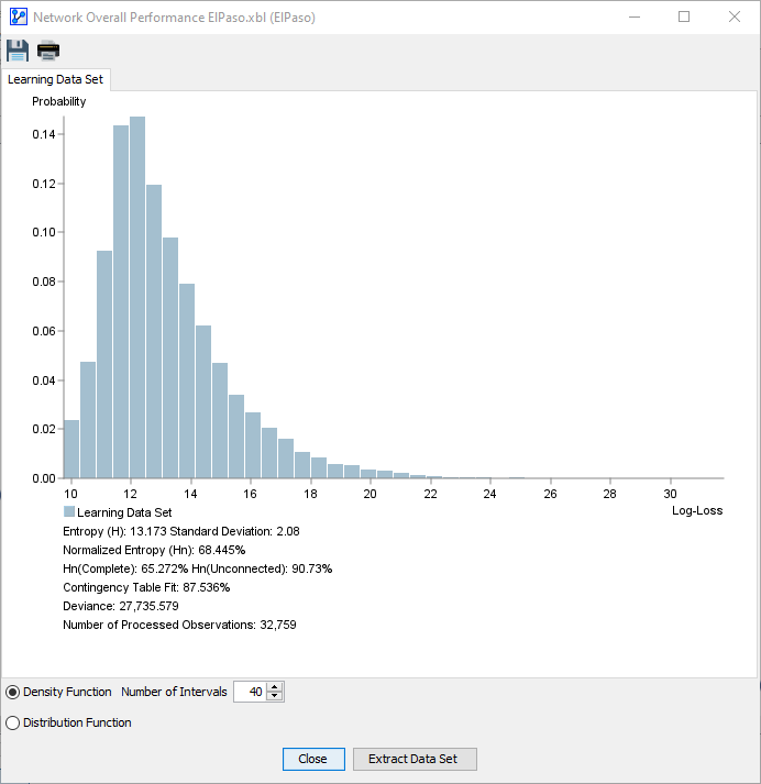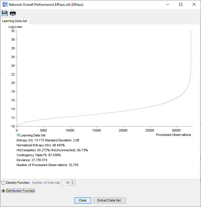The radio buttons on the bottom-left of the window allow you to switch the view between the Density function (Histogram) and the Distribution function.

Either view provides a visualization of the Log-Loss values for all observations in the dataset $D_L$ given the to-be-evaluated Bayesian network $B$ . Thus, the plots provide you with a visual representation of how well the network $B$ fits the dataset $D_L$ .

The Density view, in particular, allows you to judge the fit of the network by looking at the shape of the Log-Loss histogram.

The bars at the low end of the x-axis represented well-fitting observations. Conversely, the bars that are part of the long tail on the right represent poorly-fitting observations.

While in the Density view, you can adjust the Number of Intervals used for the histogram within a range from 1 to 100, as illustrated in the following animation:

Log-Loss

The computation of Log-Loss values is at the very core of this Overall Performance Report.

The Log-Loss value reflects the number of bits required to encode the n-dimensional evidence $E_L$ , i.e, an observation, row, or record in the dataset $D_L$ given the to-be-evaluated Bayesian network $B$ :

$L{L_B}(E_L) = - {log_2}\left( {{P_B}(E_L)} \right)$

where $P_B(E_L)$ is the joint probability of evidence E computed by the Bayesian network $B$ :

${P_B}(E_L) = {P_B}({e_1},...,{e_n})$

In other words, the lower the probability of evidence $E_L$ given the Bayesian network $B$ , the higher is the Log-Loss $LL_B(E_L)$ . As such, the Log-Loss value of an observation represents its fit to network B.

So, to produce the plots and all related metrics, BayesiaLab has to perform the following computations:

$LL_B(E_L)$ , the Log-Loss value for each observation/evidence in the Learning Set based on the learned and to be-evaluated Bayesian network B.
$LL_C(E_L)$ , the Log-Loss value for each observation/evidence in the Learning Set based on the complete network C.
$LL_U(E_L)$ , the Log-Loss value for each observation/evidence in the Learning Set based on the unconnected network $U$ .

The following Log-Loss Table is an extract of the first ten rows each from the Learning Set D_L with the computed Log-Loss values for each record:

Log-Loss Table

Evidence E from the Dataset D						Computed Values
Month	Hour	Temperature	Shortwave Radiation (W/m2)	Wind Speed (m/s)	Energy Demand (MWh)	Log-Loss (Bayesian Network)	Log-Loss (Complete Network)	Log-Loss (Unconnected Network)
						$LL_B(E_L)$	$LL_C(E_L)$	$L{L_U}(E_L)$
8	18	36.57	213.6	2	1574	13.42	15.00	22.06
8	19	36.04	105.91	1.9	1574	13.55	15.00	21.68
8	20	34.71	42.72	2.14	1485	11.93	11.68	19.4
8	21	33.94	0	2.75	1470	11.92	12.00	17.73
8	22	33.19	0	3.55	1378	11.81	11.09	17.73
8	23	32.38	0	4.21	1249	13.69	12.41	16.93
8	0	31.56	0	4.5	1110	12.91	12.19	16.93
8	1	30.6	0	4.8	1031	13.21	13.41	16.93
8	2	29.66	0	4.9	975	11.16	11.68	14.7
8	3	29.02	0	4.6	944	10.85	11.19	14.7
⁞	⁞	⁞	⁞	⁞	⁞	⁞	⁞	⁞
						$H_B(D_L)$	$H_C(D_L)$	$H_U(D_L)$
					Mean	13.17	12.56	17.46
					Std. Dev.	2.08	1.40	2.17
					Minimum	9.75	9.48	14.37
					Maximum	31.78	15.00	31.06
${log_2}({S_X}) = 19.2467$					Normalized	68.44%	65.27%	90.73%

Performance Measures

Below the plot area of the window, the Overall Performance Report shows a range of quality measures.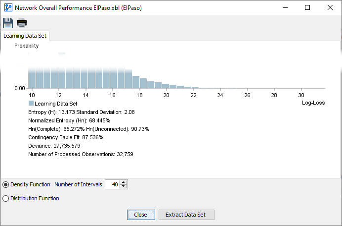

For clarity, we match up the report's labels to the notation introduced at the beginning of this topic.

Label in Report	Notation in this Topic	Explanation
Entropy (H)	$H_B(D_L)$	Mean of Log-Loss Values of all observations $E_L$ in the dataset $D_L$
Normalized Entropy (Hn)	$H_{BN}(D_L)$
Hn(Complete)	$H_{CN}(D_L)$
Hn(Unconnected)	$H_{UN}(D_L)$
Contingency Table Fit	$CTF_B(D_L)$	see Normalized Entropies
Deviance	$Dev_B(D_L)$	${Dev_B} = 2N \times \ln (2) \times \left( {{H_B}({D_L}) - {H_C}({D_L})} \right)$
Number of Processed Observations	$N(D_L)$

Entropy

The first item, Entropy $(H)$ , refers to the evaluated network $B$ . Hence, it is also denoted Entropy $H_B$ elsewhere in this topic for clarity.

More specifically, Entropy $H_B(D_L)$ is the arithmetic mean of all Log-Loss values $LL_B(E_L)$ of each observation in the dataset $D_L$ given network $B$ . In the Data Table above, Entropy $H_B(D_L)$ is highlighted.

Normalized Entropies

With Entropy not being directly interpretable as a standalone value, the report includes the Normalized Entropy $(Hn)$ . Here, Normalized Entropy $(Hn)$ also refers to the evaluated network $B$ .

Note that in the standalone topic on Entropy, we defined Normalized Entropy on the basis of a single variable with one set of states.

Here, however, we need to consider that we have several variables with differing numbers of states. So, we require a more general definition of Normalized Entropy:

where

$\cal X$ is the set of variables in network $B$ .
is the size of the Joint Probability Distribution, i.e., the number of state combinations defined by all variables in $B$ .

With that, can calculate the value:

${H_{BN}}({\cal X}) = \frac{{{H_B}({\cal X})}}{{{{\log }_2}({S_{\cal X}})}} = \frac{{{13.1733}}}}{{{19.2467}}}} = 68.44\%$

Furthermore, the report provides the Normalized Entropies for a complete (fully-connected) network $C$ and the unconnected network $U$ .

Complete (Fully-Connected) Network $C$

$H_n(Complete)$ refers to the Normalized Entropy computed from all observations with a complete network $C$ (depicted below), which is the best-fitting representation of the observations.

Unconnected Network $U$

$H_n(Unconnected)$ is the Normalized Entropy obtained with an unconnected network $U$ , which is the worst-fitting representation of the observations.

Contingency Table Fit (CTF)

Contingency Table Fit (CTF) measures the quality of the representation of the Joint Probability Distribution by a Bayesian network $B$ in comparison to a complete network $C$ .

BayesiaLab's CTF is defined as:

where

$H_U(\mathcal{D})$ is the entropy of the dataset with the unconnected network $U$ .
$H_B(\mathcal {D})$ is the entropy of the dataset with the network $B$ .
$H_C(\mathcal {D})$ is the entropy of the dataset with the complete network $C$ .

Interpretation

$C_B$ is equal to 100 if the Joint Probability Distribution is represented without any approximation, i.e., the entropy of the evaluated network $B$ is the same as the one obtained with the complete network $C$ .
$C_B$ is equal to 0 if the Joint Probability Distribution is represented by considering that all the variables are independent, i.e., the entropy of the evaluated network $B$ is the same as the one obtained with the unconnected network $U$ .
$C_B$ can also be negative if the parameters of network $B$ do not correspond to the dataset.
The dimensions represented by Not-Observable Nodes are excluded from this computation.

Deviance

The Deviance measure is based on the difference between the Entropy of the to-be-evaluated network $B$ and the Entropy of the complete (i.e., fully-connected) network $C$ .

Definition

Deviance is formally defined as:

${D_B} = 2N \times \ln (2) \times \left( H_B(\mathcal {D}) - H_C(\mathcal {D}) \right)$

where

$H_B(\mathcal {D})$ is the Entropy of the dataset given the to-be-evaluated network $B$ .
$H_C(\mathcal {D})$ is the Entropy of the dataset given the complete (i.e., fully-connected) network $C$ .
$N$ is the size of the dataset.

Using the values from the Data Table above, we obtain:

${D_B} = 2N \times \ln (2) \times \left( {{H_B} - {H_C}} \right) = 2 \times 32,759 \times 0.6932 \times 13.1733 - 12.5627 = 27,735.579$

Interpretation

The closer the Deviance value is to 0, the better the network $B$ represents the dataset.

Report Footer

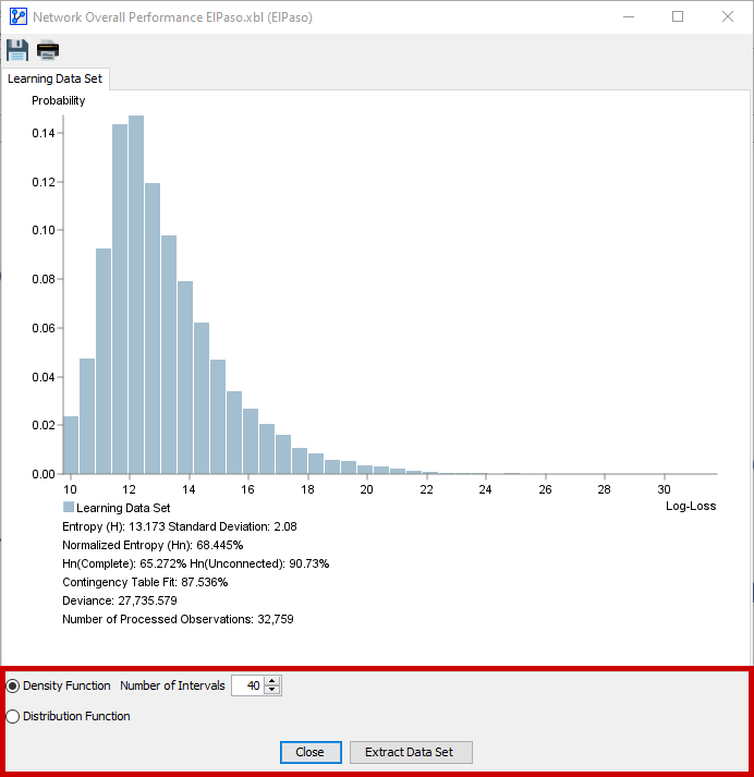
Extract Data Set

The final element in the report window is the Extract Data Set button. This is a practical tool for identifying and examining outliers, e.g., those at the far end of the right tail of the histogram.

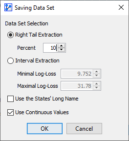
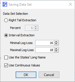
Clicking the Extract Data Set button brings up a new window that allows you to extract observations from the dataset according to the criteria you define:
Right Tail Extraction selects the specified percentage of observations, beginning with the highest Log-Loss value.
Interval Extraction allows you to specify a lower and upper boundary of Log-Loss values to be included.
Upon selecting either method and clicking OK, you are prompted to choose a file name and location.
BayesiaLab saves the observations that meet the criteria in CSV format.
Note that the Log-Loss values that are used for extraction are not included in the saved dataset.