Data Clustering

Context

Data Clustering is a type of unsupervised learning algorithm that creates a new node, [Factor_i].
Each state of this newly-created node represents a Cluster.
Data Clustering can be used for different purposes:
- For finding observations that appear the same, i.e., have similar values.
- For finding observations that behave the same, i.e., interact similarly with other nodes in the network.
- For representing an unobserved dimension by means of an induced latent Factor.
- For summarizing a set of nodes.
- For compactly representing the Joint Probability Distribution.
From a technical perspective, each cluster should be:
- Homogeneous and pure.
- Clearly differentiated from other clusters.
- Stable.
From a functional perspective, all clusters should be:
- Easy to understand.
- Operational.
- A fair representation of the data.
Data Clustering with Bayesian networks is typically based on a Naive Bayes structure, in which the newly-created latent Factor Node [Factor_i] is the parent of the so-called Manifest Nodes.
- latent (adjective): (of a quality or state) existing but not yet developed or manifest; hidden or concealed.
- manifest (adjective): clear or obvious to the eye or mind.
This variable being hidden, i.e., with 100% of missing values, the marginal probability distribution of [Factor_i] and the conditional probability distributions of the Manifest variables are initialized with random distributions.
Thus, an Expectation-Maximization (EM) algorithm is used to fit these distributions with the data:
- Expectation: the network is used with its current distributions for computing the posterior probabilities of [Factor_i], for the entire set of observations described in the data set; These probabilities are used for soft imputing [Factor_i];
- Maximization: based on these imputations, the distributions of the network are updated via Maximum-Likelihood. The algorithm goes back to Expectation until no significant changes occur to the distributions.

Usage

You can either select a subset of nodes to be included in Data Clustering, or leave all node unselected. In the latter case, all nodes on the [Graph Panel](/Users/stefanconrady/Library/CloudStorage/OneDrive-BayesiaUSA/ClickHelp Backup/project-backup_bayesialab_2024-06-07_08-24-26/HTML/graph-windows-graph-panel.html) will be included for Data Clustering.

Feature History

[Data Clustering] has been updated in versions [5.1]and [5.2].

New Feature: Meta-Clustering

This new feature has been added for improving the stability of the induced solution (3_rd technical quality). It consists of creating a dataset made of a subset of the Factors that have been created while searching for the best segmentation, and using Data Clustering on these new variables. The final solution is thus a summary of the best solutions that have been found (4^th purpose).

The five Manifest variables (bottom of the graph) are used in the dataset for describing the observations.

The Factor variables [Factor_1], [Factor_2], and [Factor_3] have been induced with Data Clustering. They are** then imputed to create a new dataset.

In this example, three Factor variables are used for creating the final solution [Factor_4].

Example

Let's use a dataset that contains house sale prices for King County (opens in a new tab), which includes the city of Seattle, Washington. It describes homes sold between May 2014 and May 2015. More specifically, we have extracted 94 houses that are more than 100 years old, that have been renovated, and come with a basement. For simplicity, we are just describing the houses with the 5 Manifest variables below, discretized into 2 bins.

grade: Overall grade given to the housing unit
sqrt_above: Square footage of house, apart from basement
sqft_living15: Living room area in 2015
sqft_lot: Square footage of the lot
lat: Latitude coordinate

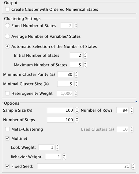
The wizard below shows the settings used for segmenting these houses:

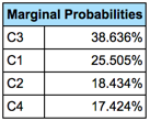
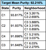
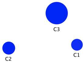
After 100 steps, segmenting the houses into 4 groups is the best solution. Below, the Mapping function shows the newly created states/segments:

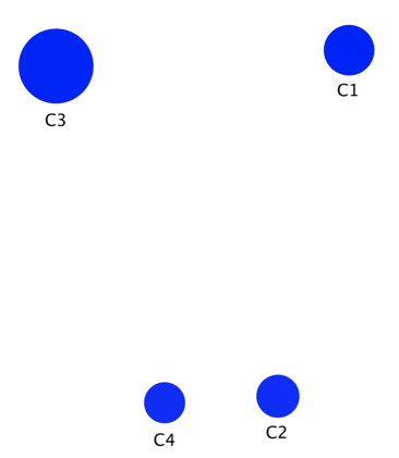
the size of each segment is proportional to its marginal probability (i.e. how many houses belong to each segment),
the intensity of the blue is proportional to the purity of the associated cluster (1^st technical quality), and
the layout reflects the neighborhood.

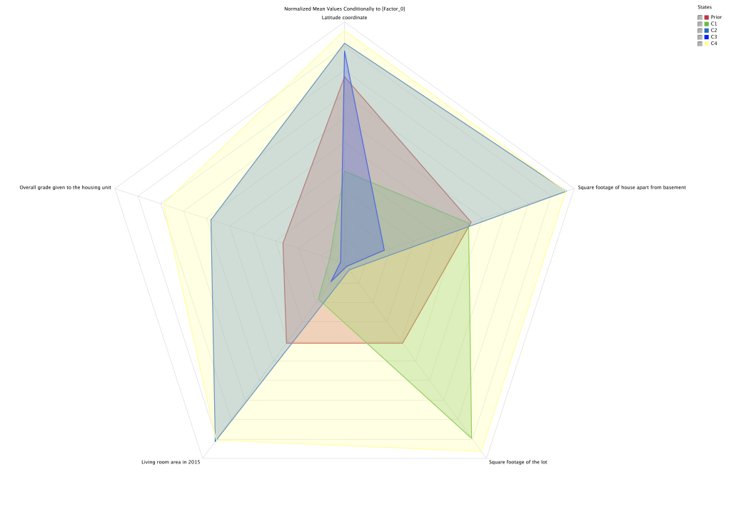
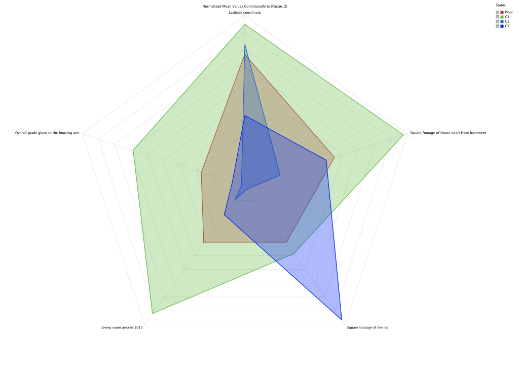
This radar chart (Menu > Analysis > Report > Target > Posterior Mean Analysis > Radar Chart) allows interpreting the generated segments. As we can see, they are easily distinguishable (2^nd technical quality).

Thus, the solution with 4 segments satisfies the first two technical qualities listed above. However, what about the 3_rd one, the stability? Below are the scores of the 10 best solutions that have been generated while learning:

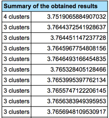
Even though the best solution is made of 4 segments, this is the only solution with 4 clusters, all the other ones have nearly the same score, but with 3 clusters. Thus, we can assume that a solution with 3 clusters would be more stable.

Using Meta-Clustering on the 10 best solutions (10%) indeed generates a final solution made of 3 clusters.

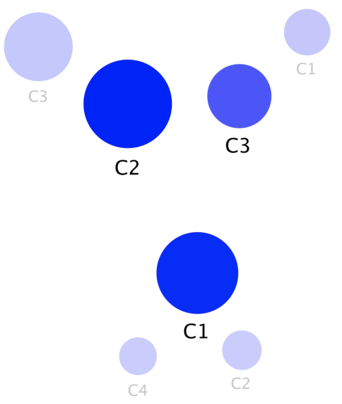
This mapping juxtaposes the mapping of the initial solution with 4 segments (lower opacity) and of the one corresponding to the meta-clustering solution.

The relationships between the final and initial segments are as follows:

C1 groups C4 and C2 (the main difference between C4 and C2 was Square footage of the lot),
C2 corresponds to C3
C3 corresponds to C1

New Feature: Multinet

As stated in the Context, Data Clustering with Bayesian networks is typically done with Expectation-Maximization (EM) on a Naive structure. Thus, it is based on the hypothesis that the Manifest variables are conditionally independent of each other given ***[Factor_i]_**. Therefore, the Naive structure is well suited for finding observations that look the same (1^st purpose), but not so good for finding observations that behave similarly (2^nd purpose). The behavior should be represented by direct relationships between the **Manifests**.

Our new Multinet clustering is an EM² algorithm based both on a Naive structure (Look) and on a set of Maximum Weight Spanning Trees (MWST) (Behavior). Once the distributions of the Naive are randomly set, the algorithm works as follows:

Expectation_Naive: the Naive network is used with its current distributions for computing the posterior probabilities of [Factor_i], for the entire set of observations described in the data set; These probabilities are used for hard-imputing [Factor_i], i.e. choosing the state with the highest posterior probability;
Maximization_MWST: [Factor_i] is used as a breakout variable. An MWST is learned on each subset of data.
Expectation_MWST: the joint probabilities of the observations are computed with each MWST and used for updating the imputation of [Factor_i].
Maximization_Naive: based on this updated imputation, the distributions of the Naive network are updated via **Maximum-Likelihood. Then, the algorithm goes back to Expectation_Naive, until no significant changes occur to the distributions.

Two parameters allow changing the Look/Behavior equilibrium. They can be considered as probabilities to run the Naive and MWST steps at each iteration.

Setting a weight of 0 for Behavior defines a Data Clustering quite similar to the [usual one](/Users/stefanconrady/Library/CloudStorage/OneDrive-BayesiaUSA/ClickHelp Backup/project-backup_bayesialab_2024-06-07_08-24-26/HTML/18351067.html#DataClustering(7.0)-EM1718232680), but based on hard imputation instead of soft imputation.

Example

Let's use the same data set that describes houses in Seattle.

The wizard below show the settings we used for segmenting the houses:

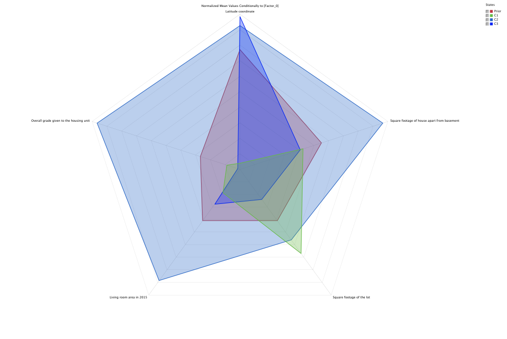
After 100 steps, segmenting the houses into three groups is the best solution. The final network is a Naive Augmented Network, with a direct link between two Manifest variables, which are, therefore, not independent given the segmentation, i.e. the Behavior part. Note that this dependency is valid for C3 only, which can be seen after performing inference with the network.

The radar chart allows analyzing the Look of the segments.

New Feature: Heterogeneity Weight

The assumption that the data is homogeneous, given all the Manifest Variables, can sometimes be unrealistic. There may be significant heterogeneity in the data across unobserved groups, and it can bias the machine-learned Bayesian networks. This phenomenon is known as Unobserved Heterogeneity, i.e. an unobserved variable in the dataset.

Data Clustering represents a solution for searching for such hidden unobserved groups (3^rd purpose). However, whereas the default scoring function in Data Clustering is based on the entropy of the data, finding heterogenous groups requires modifying the scoring function.

We thus defined a Heterogeneity Index :

with

where:

is the induced Factor,
are the states of the Factor, i.e. the segments used to split the data,
is the marginal probability of state , i.e. the relative size of the segment,
is the set of Manifest variables,
is the entire data set,
is the subset of the data that corresponds to the segment
is the Mutual Information between the Manifest variable and the Target Node computed on the data set .

The Heterogeneity Weight allows setting a weight of the Heterogeneity Index in the score, which will, therefore, bias the selection of the solutions toward segmentations that maximize the Mutual Information of the Manifest variables with the Target Node.

Example

Let's use the entire data set that describes houses in Seattle, with this subset of Manifest variables:

Renovated: indicates if the house has been renovated
Age: Age of the house
sqft_living15: Living room area in 2015
long: Longitude coordinate
lat: Latitude coordinate
Price (K$): Price of the house**.**

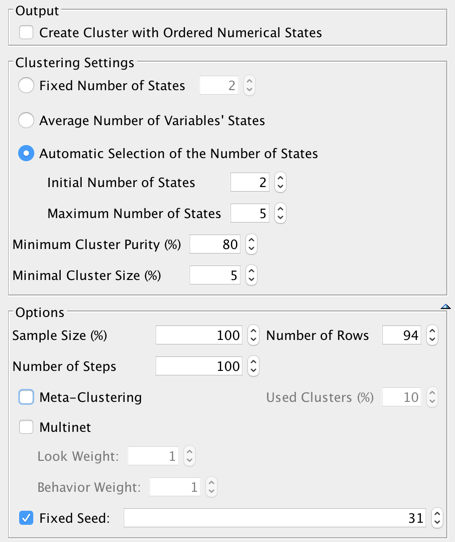
After setting Price (K$) as a Target Node and selecting all the other variables, we use the following settings for Data Clustering:

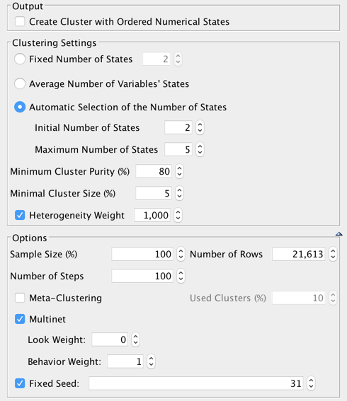
This returns a solution with 2 segments, generating a Heterogeneity Index of 60%. This indicates, therefore, that using [Factor_i] as a breakout variable would increase the sum of the Mutual Informations of the Manifest variables with the Target Node by 60 %.

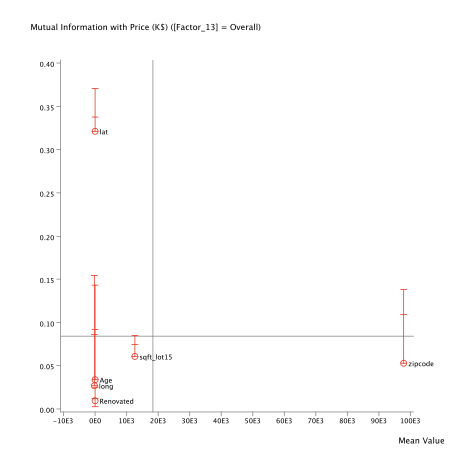
The Quadrant Chart below highlights the improvement of the Mutual Information. The points correspond to the Mutual Informations on the entire data set, and the vertical scales show the variations of the Mutual Informations by splitting the data based on the values of ***[Factor_i]._**

The Heterogeneity Index is computed on the Manifest variables that are used during the segmentation only. In order to take into account other variables in the computation of the index, these variables have to be included in the segmentation, with a weight of 0 for preventing them to influence the segmentation.

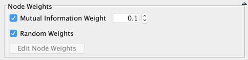
New Feature: Random Weights

By default, the weight associated with a variable is set to 1. Whereas a weight of 0 renders the variable purely illustrative, a weight of 2 is equivalent to duplicating the variable in the dataset. The option [Mutual Information Weight,](/Users/stefanconrady/Library/CloudStorage/OneDrive-BayesiaUSA/ClickHelp Backup/project-backup_bayesialab_2024-06-07_08-24-26/HTML/2851547.html) introduced in version 5.1, allows weighting the variable by taking into account its Mutual Information with the Target node.

As of version 7.0, a new option, Random Weights, allows to modify the weight values randomly while trying the find the best segmentation. The amplitude of the randomness is inversely proportional to the current number of trials, therefore starting with the maximum level of randomness and ending with almost no weight modification. This option can be useful for escaping from local minima.

Binary Clustering K Means