Mosaic Analysis
Context
- BayesiaLab’s Mosaic Analysis can produce high-dimensional Mosaic Plots to visualize marginal and conditional distributions of nodes in a Bayesian network.
- Mosaic Analysis is a useful tool for creating a data overview and highlighting dependencies between nodes, or the lack thereof.
- The Mosaic Analysis can also display Standardized Pearson Residuals, which are computed for all cells in the plot. For easy comparison, all cells are color-coded using Standardized Pearson Residuals.
Usage
-
To illustrate the basic display and layout options of the Mosaic Analysis, we use an arbitrary Bayesian network with four nodes, N1 through N4, which you can download here:
GenericNetwork.xbl -
To start the analysis, select one or more nodes.
-
Then, go to
Main Menu > Analysis > Visual > Overall > Mosaic. -
A new window opens up offering you a number of settings:
Variables
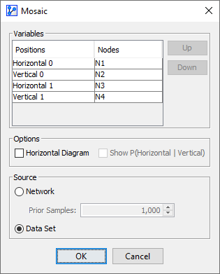
- The nodes we originally selected on the Graph Panel are now shown in the Variables tables:
Loading SVG...
Note that we refer to both Nodes and Variables here. This is because we can analyze the probabilities on the basis of the states of the Nodes in the network or, if available, on the data recorded in the original Variables.
- You can reassign the Nodes to different Positions by using the Up and Down buttons.
Options
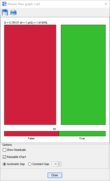
- Under Options, you can configure the overall layout of the Mosaic Plot given the number of available nodes.
Number of Variables/Dimensions |  |  |  |
|---|---|---|---|
1 | Loading SVG... | n/a | n/a |
|  |
|
|
2 | Loading SVG... | Loading SVG... | Loading SVG... |
|  |  | 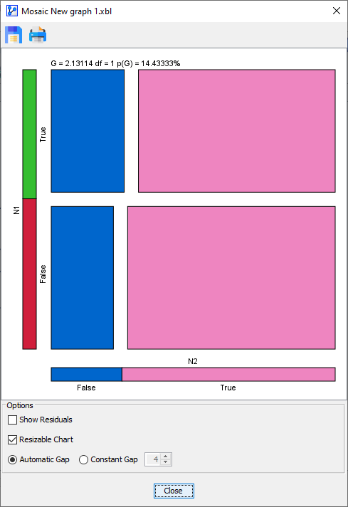 |
3 | Loading SVG... | Loading SVG... | Loading SVG... |
| 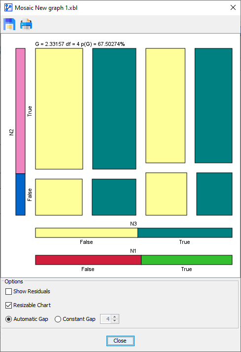 | 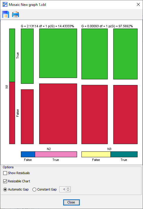 | 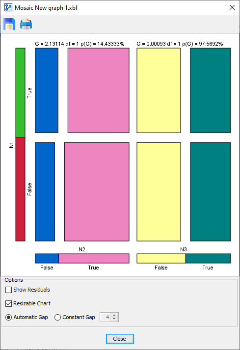 |
4 | Loading SVG... | Loading SVG... | Loading SVG... |
| 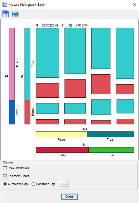 | 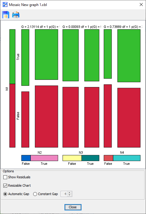 | 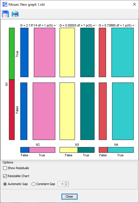 |
Source
-
The Source Panel at the bottom of the window allows you to choose the basis for generating the Mosaic Plot.

-
One of the key features of the Mosaic Analysis is the ability to generate statistical measures for augmenting the visual presentation.
-
This is possible for Bayesian networks with and without an associated dataset:
- If a dataset is associated with your network, you can choose the Source, i.e., the Dataset or the Network.
- Dataset: the Standardized Pearson Residual is computed with the associated dataset.
- If there are Hidden Nodes in the network, i.e., nodes without any corresponding data, the Mosaic Analysis defaults to Network as a source.
- If the associated dataset contains Learning Set/Test Set split, you can select either subset or all observations.
- Network: BayesiaLab uses the given network to generate a dataset from which the Standardized Pearson Residual can be computed.
- In the Prior Samples field, you need to specify the number of observations or samples to be generated.
- If no dataset is associated with your network, only the Network option is available as a Source for the Mosaic Analysis.
-
Beyond the Mosaic Analysis settings that we explained in the above section, we illustrate the complete Mosaic Analysis workflow in the following example.
Usage Example
-
To explain the Mosaic Analysis workflow in more detail, we use a Bayesian network that represents the relationship between Hair Color, Eye Color, and Sex. You can download the network here:
HairColorEyeColorSex.xbl -
For this analysis, we select all three nodes, i.e., Hair Color, Eye Color, and Sex.
-
Then, go to
Main Menu > Analysis > Visual > Overall > Mosaic.
Configuration
-
The configuration window opens.

-
The above settings specify that:
- Sex is the first horizontal variable (Horizontal 0 or H0).
- Hair Color is the first vertical variable (Vertical 0 or V0)
- Eye Color is the second horizontal variable (Horizontal 1 or H1)
-
Furthermore, the Options panel includes a Reference Model section, which only applies to analyses with precisely 3 variables. However, we defer the discussion and will include it in a dedicated section about the Standardized Pearson Residual.
Mosaic Plot
-
Upon clicking OK, the Mosaic Plot window opens up with a colorful mosaic.

-
The bar at the very bottom of the plot represents the marginal distribution of Sex. The length of each section is proportional to the marginal probability of the corresponding state. Given the near 50/50 split of male and female subjects in the dataset, the red and green bars have almost the same length.
Loading SVG... -
The bar closest to the mosaic represents the marginal distribution of Eye Color. Here, the differences in marginal probabilities are more prominent.
Loading SVG... -
The vertical bar to the left of the mosaic represents the marginal distribution of Hair Color.
Loading SVG... -
The size or area of each cell in the main area of the Mosaic Plot is proportional to the Joint Probability of the states that correspond to that cell in the plot area, i.e., , which is in our example .
-
Furthermore, the width of each cell is proportional to the conditional probability
, i.e., .
-
Finally, the height of each cell is proportional to
, i.e., .
Tooltip
-
As there are no labels on the cells, you can bring up all cell-specific information in Tooltips.
-
Whenever you hover over any of the cells with your cursor, a Tooltip appears, like the one below:

-
For instance, the cell under the cursor in the following screenshot represents the Joint Probability .
-
Note that, in this context, the comma (”,”) represents the conjunction AND.

-
Each Tooltip includes the following items:
-
The states that correspond to the Joint Probability, e.g., , , , which is the cell in the upper left-hand corner of the plot.
-
The value of the Joint Probability, . Given the size constraint of the Tooltip, this expression is shown in abbreviated form, i.e., .
-
The Conditional Probability , i.e., the probability of GIVEN THAT AND . Note that the vertical bar "" means “given that.”
-
The size of the corresponding population in the dataset, i.e., Population=7. So, 7 out of 592 cases are females, have blue eyes and red hair.
- In this example, we generated the Mosaic Plot from an attached dataset.
- However, we could have produced the plot on the basis of the network only, using simulated data. For instance, had we created 1,000 Prior Samples, the corresponding blue/red/female population would be 11.8, i.e., 1.18% of the overall population of 1,000 Prior Samples.
-
The D-Value shown in the Tooltip represents the Standardized Pearson Residual of the cell. We discuss the D-Value and Standardized Pearson Residual in the following section.
-
Independence Tests & Standardized Pearson Residual
- The Mosaic Analysis provides test statistics on two levels:
-
Overall Statistics: With the Mosaic Plot, BayesiaLab performs an independence test -Test or G-Test for all variables in the analysis.
-
You can specify which test to use under
Main Menu > Window > Preferences > Tools > Statistical Tools. -
The selected test statistic is shown at the top of the Mosaic Plot window, including the degrees of freedom and the significance level.
Loading SVG... -
With this -value and the shown degrees of freedom, the null hypothesis (i.e., the cells are independent) would be rejected at a 0% significance level.
-
For the remainder of this section, all statistical measures are based on the -Test.
-
-
Cell-Specific Statistic: For each cell in the Mosaic Plot, BayesiaLab computes the Standardized Pearson Residual, denoted .
-
The Standardized Pearson Residual captures each cell’s departure from its expected value and, thus, quantifies any potential over- or under-representation of a particular cell in the Mosaic Plot relative to the Null-Hypothesis.
-
It is defined as follows:
where and represent the observed and expected values of cell .
-
The value of is included in the information provided in the Tooltip.
-
Additionally, can be specifically visualized in an alternate view of the Mosaic Plot, i.e., the Residuals Plot.
-
-
Residuals Plot
-
To switch to the Residuals Plot, check the Show Residuals checkbox at the bottom of the Mosaic Plot window.
-
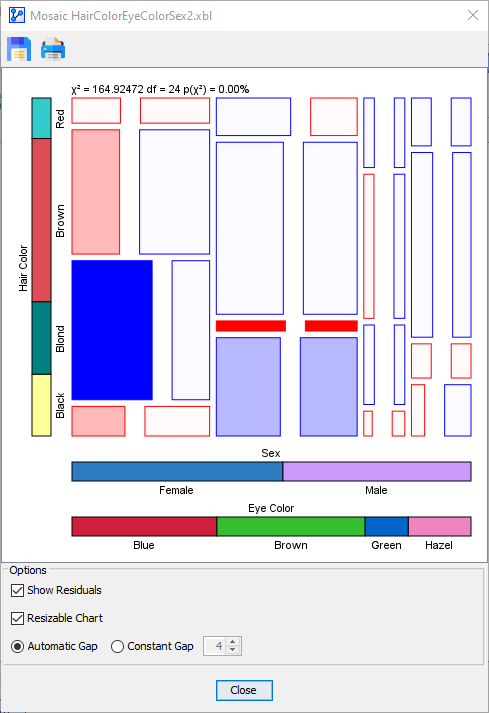
Now the color-coding of the cells corresponds to the Standardized Pearson Residual ():
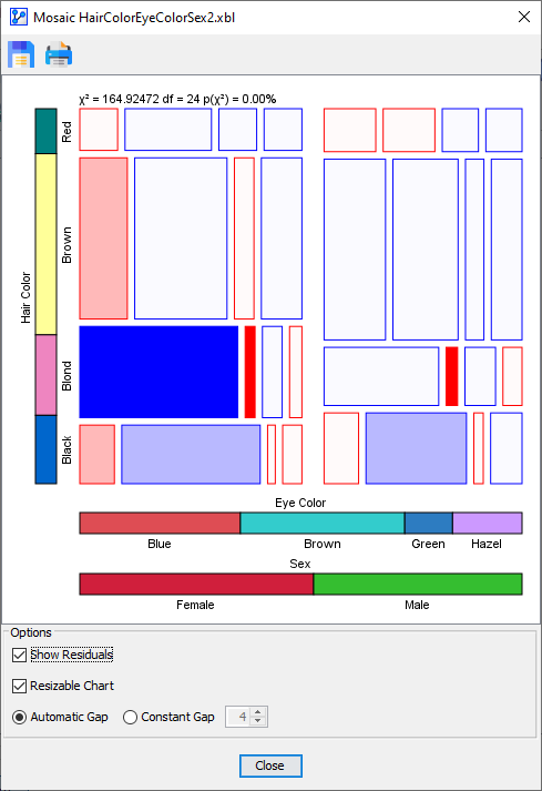

: very significant over-representation

: significant over-representation

: no significant over-representation

: no significant under-representation

: significant under-representation

: very significant under-representation

Denotes the absence of observations in the dataset or the simulated data.
-
In the above Residuals Plot, the most notable over-representation is for with . In other words, for females, there is a significant positive correlation between blue eyes and blond hair.
-
The adjacent cell, i.e., , is an example of very significant under-representation with . This means that, for females, there is a significant negative correlation between brown eyes and blond hair.
Null-Hypothesis Options for Three-Dimensional Plots
-
For three-dimensional plots only, the Mosaic Analysis offers options that are not available in any other context.
-
If you select three nodes to be included in the Mosaic Analysis, the configuration window offers an additional option:

-
Under Reference Model, you can select between the three structures that represent the Null-Hypothesis:
- H0, H1, and V0 are all independent nodes, i.e., an unconnected network.
- H0 and H1 are dependent, while V0 is independent.
- H0 and H1 are dependent, plus H0 and V0 are dependent. H1 and V0 are conditionally independent.
-
With that, we can focus on investigating the relationships of specific variables.
-
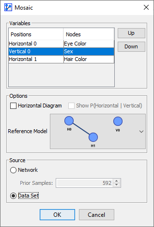
For instance, now that we have learned about the significant correlation between Eye Color and Hair Color, we can specifically test for the independence of Sex.
-
In the variables list, we move Sex to Position V0 and select the corresponding Reference Model.
-
The Residual Plot shows the results:

-
We see that on the basis of the -Test, we cannot reject the Null-Hypothesis that Sex is independent.
-
However, values of -2.15 and 2.03 respectively suggest that, given blue eyes, blond hair is still under-represented among males and over-represented for females.
-
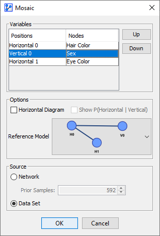
On this basis, we can revisit the Null-Hypothesis and now speculate that Eye Color is independent of Sex conditional on Hair Color. We arrange the variables accordingly in the Variables list.
-
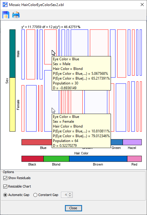
Indeed, the Residual Plot appears to confirm our speculation:
-
We see that on the basis of the -Test, we cannot reject the Null-Hypothesis that Sex and Eye Color are independent conditional on Hair Color.
-
As indicated by the Tooltips, all D values are now within the non-significant range.
Display Options
-
At the bottom of the Mosaic Plot window, there are additional options regarding the styling of the Mosaic Plot.
-
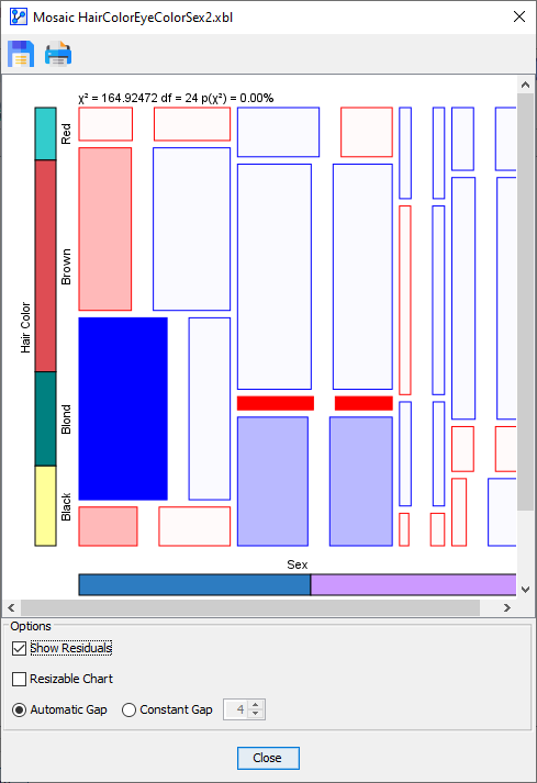
With the Resizable Chart option engaged, you can resize the Mosaic Plot window and the Mosaic Plot itself will adjust automatically while maintaining the proportionality of probabilities and cell areas.
-
With the Resizable Chart option disabled, the Mosaic Plot will be of a fixed size. As a result, you may need to resize the window or use the scrollbars to see the entire plot.
-
The last option affects the size of the gaps between the cells in the plot:
- Automatic Gap
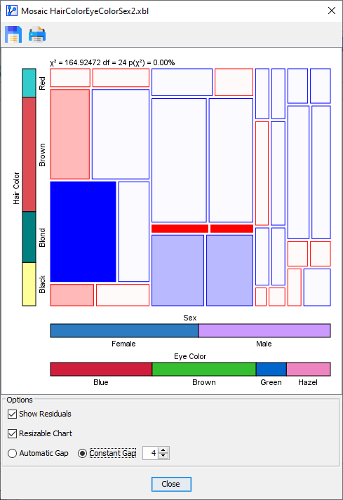
- Constant Gap: You can specify the gap width between the cells in pixels.
-
The following table compares the two gap options side-by-side.
Automatic Gap
Constant Gap
